
Google Sheets lets you sort Pivot Tables by row fields, column fields, or summarized values. The available sorting options depend on the Pivot Table layout and the fields used for grouping.
In this tutorial, you’ll learn how to sort Pivot Tables grouped by a single row field, multiple row fields, and both rows and columns. We’ll also see how the available sorting options differ in each case.
This tutorial covers the built-in value-based sorting options. If you want a custom sort order (for example, status values such as Under Progress → Completed → Withheld), see the custom-order tutorials linked below.
Quick Steps
You can follow these quick steps to sort Pivot Table rows or columns by values in Google Sheets.
- Open the Pivot Table editor.
- Go to the Rows or Columns section.
- Under Sort by, choose the field or summarized value.
- Under Order, choose Ascending or Descending.
The available Sort by options depend on the Pivot Table layout. The following examples show how they change as you add row and column fields.
Sort a Pivot Table by Value When Grouped by Rows
Assume you have the following sales data.
| Region | Product | Sales |
|---|---|---|
| East | Monitor | 7500 |
| East | Mouse | 6400 |
| East | Laptop | 15000 |
| … | … | … |
For the complete dataset and the Pivot Tables used in this tutorial, make a copy of my sample Google Sheets file.
First, create a Pivot Table by adding Region to the Rows field and Sales to the Values field in the Pivot Table editor.
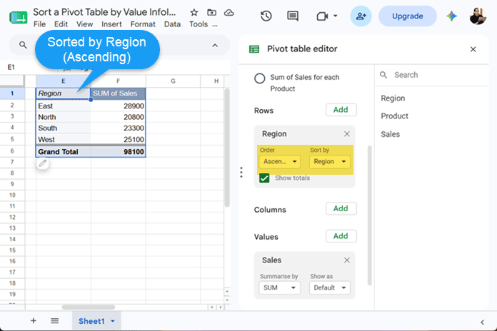
In the Pivot Table editor, you can sort the Region row field in two ways:
- By Region in alphabetical ascending or descending order.
- By the Sum of Sales for each region in ascending or descending order.
That’s all there is to it when your Pivot Table contains a single row field.
Now, let’s add one more field to the row grouping by adding Product below Region in the Rows field.
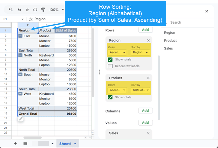
This time, you’ll get sorting options for both row fields, allowing multi-level sorting. You should understand what each option does, as they can be misleading.
Let’s start with the top-level row field, Region. Sorting by Region works exactly as before—it sorts the regions alphabetically in ascending or descending order. Sorting by Sum of Sales, however, sorts the regions based on their total sales, not the individual products within each region.
When it comes to Product, you can sort the products alphabetically in ascending or descending order within each region. If you choose Sum of Sales, the products are sorted by their sales values, again within each region.
Understanding this difference is essential when sorting Pivot Table rows by value in Google Sheets.
Note: The available Sort by options depend on your Pivot Table layout. Your Pivot Table may not display every option shown in this tutorial if it uses a different row or column grouping.
Sort a Pivot Table by Value When Grouped by Rows and Columns
This time, add Product to the Rows field, Region to the Columns field, and keep Sales in the Values field.
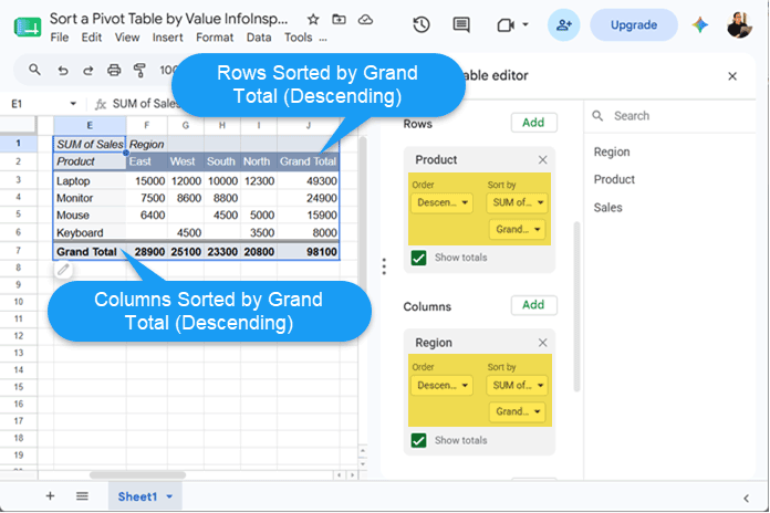
With both row and column groupings, Google Sheets provides several options for sorting the Pivot Table by values.
Sort Pivot Table Rows by Value
Let’s start with the Rows field, which sorts the Pivot Table rows in ascending or descending order.
You will see two primary Sort by options:
- Product
- Sum of Sales
Product
Sorts the rows alphabetically by product name in ascending or descending order.
Sum of Sales
Provides additional options, including Grand Total and each individual region.
- Selecting Grand Total sorts the rows based on the values in the Grand Total column.
- Selecting a region (for example, East) sorts the rows based on the values in that region’s column.
Tip: If you want to arrange the Pivot Table rows in a custom order instead of sorting them alphabetically or by values, see How to Sort Pivot Table Rows in Custom Order in Google Sheets.
Sort Pivot Table Columns by Value
The Columns field provides similar sorting options, but they apply to the Pivot Table columns.
You will see two primary Sort by options:
- Region
- Sum of Sales
Region
Sorts the column labels alphabetically in ascending or descending order.
Sum of Sales
Also provides additional options, including Grand Total and each individual product.
- Selecting Grand Total sorts the columns based on the values in the Grand Total row.
- Selecting a product (for example, Laptop) sorts the columns based on the values in that product’s row across all regions.
Tip: If you want to display the Pivot Table columns in a custom order instead of sorting them alphabetically or by values, see How to Sort Pivot Table Columns in Custom Order in Google Sheets.
Frequently Asked Questions
Does unchecking “Show totals” disable sorting by Grand Total?
No. Even if you hide the Grand Total row or column by unchecking Show totals, you can still sort the Pivot Table by the Grand Total values.
Why do I see different sorting options in my Pivot Table?
The available sorting options depend on the Pivot Table layout and the level of row or column grouping. As you add or remove row and column fields, Google Sheets updates the available Sort by options based on the current grouping structure.
Key Takeaways
Once you understand how Google Sheets determines the available Sort by options, sorting Pivot Tables becomes straightforward. Whether you’re sorting row fields, column fields, Grand Totals, or summarized values, the available options depend on your Pivot Table’s grouping structure.
If you’re not familiar with functions such as QUERY or SUMIFS, a Pivot Table is often the simplest way to summarize and analyze your data.
To learn more about Pivot Tables, check out these guides: