There is no built-in option to sort Pivot table columns in a custom order in Google Sheets. We should follow a workaround for that.
In Pivot table reports, other than sorting columns and rows in ascending/descending order, I think there must be a custom sort order.
Honestly, I am unhappy with the sort order of columns in a Pivot table report.
Because even if we are not satisfied with the ascending or descending sort order, we can’t manually change the column order by drag and drop.
You may try to manually drag and drop the columns to get your desired column order. Nothing will happen (earlier, it was returning the #REF error).
I forgot to say one thing! Other than sorting Pivot table columns in ascending or descending order, there is one more option. That is sorting the columns by the Grand Total.
Want to master Pivot Table sorting and filtering? Check out our full guide: How to Sort and Filter Pivot Tables in Google Sheets. It covers custom column orders, grand total sorting, and more advanced techniques.
In this tutorial, let’s learn to sort Pivot table columns in a custom list order in Google Sheets.
Pivot Table Default Output Without Custom Sorting of Columns:
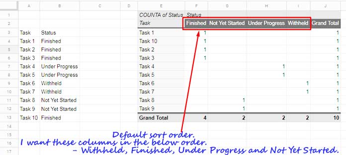
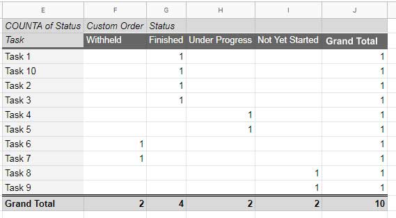
In the above Pivot Table, I have entered the custom order list (in blue ink). In that order, I want the columns to appear. See that customized table below.
Pivot Table Field (Column) Labels Sorted by Custom Order:
Steps to Sort Pivot Table Columns in Custom Order in Google Sheets
My workaround uses an additional column (helper column).
In my above example, the source data is in the range A3:B. Please refer to the first screenshot to see the sample data.
The first column contains task names, and the second column contains its current statuses.
We want to get the count of finished, under progress, withheld, and not yet started tasks. For that, we will use the Pivot table feature in Google Sheets.
See the Pivot Table report (in the first screenshot). You can see that the status column (B3:B) in the source data is pivoted (arranged in columns).
The field labels in the Pivot table are the unique values from this column sorted in A-Z order.
Now let me begin with the steps to Sort Pivot Table Columns in Custom Order in Google Sheets.
Step 1: Helper Column for Pivot Table that Contains Custom Sort Order Numbering
In cell C3, I am going to use the below array formula. So, the range C3:C13 will act as a helper column in the report.
=ArrayFormula({"Custom Order";IFERROR(match(B4:B,{"Withheld";"Finished";"Under Progress";"Not Yet Started"},0))})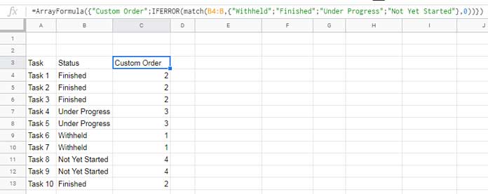
The Formula Logic:
The Pivot table custom sort order is based on the status column B because the unique values from this column will be the field labels in the report.
So the above Match formula uses values in that column as the search keys and the custom order values (list) as the range.
It can make you confuse. So, first, see the syntax of the Match function and the generic formula.
Syntax:
MATCH(search_key, range, [search_type])Generic Formula:
MATCH(status column B, custom sort order values, 0)Now, please check my above Match formula. I hope you can understand that better now.
If you face issues understanding the above Match-based formula, please don’t hesitate to ask me in the comment below.
Step 2: Settings in Pivot Table Editor to Sort Pivot Table Columns in the Custom Order
First, select the range A3:C13. Then go to the Insert menu Pivot table.
Where do you want the report? You can either have it in the existing sheet or a new sheet.
I prefer it in the current sheet cell E1. So check “Existing sheet” and enter E1 in the corresponding field. Click on the “Create” button.
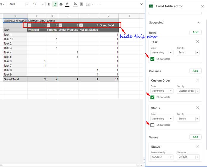
The settings inside the Pivot table editor:
- Rows > Add > Task.
- Columns > Add > Custom Sort Order (the Helper column).
- Columns > Add > Status (uncheck “Show totals”)
- Values > Add > Status > Summarise by > COUNTA.
Please refer to the following image to understand these Pivot table editor settings better.
Step 3: Additional Manual Settings in the Pivot Table Report
There are two additional settings, and both of them are optional.
First, hide row # 2 (see the image above) in the report containing the sort order label.
Then use the Insert menu Drawing to create a text box containing the text “Grand Total”. Change the font color to white and place it in cell J3 as below.
That’s it! You can follow this workaround to sort Pivot table columns in the custom order in Google Sheets.


For the Column E, how do we fix that? Task 10 comes right after Task 1
Hi, Chanelle Marcelo,
In cell D3, insert the following formula.
={"Sort";ArrayFormula(ifna(REGEXEXTRACT(A4:A&"","[0-9]+")*1))}Make the following two changes within the pivot table editor panel.
1. Modify the range to A3:D1000.
2. Add the new column under Add Rows.