


How to create a month-wise Pivot Table report in Google Sheets? If the data has a “Month” column, this topic will not be dealt with here. Anyone can easily group that column like a category column.
I want to create a pivot table that summarises the data month-wise. But my data has no month column. Instead, it has a column with dates.
So it’s all about grouping a date column by month in the Pivot table in Google Sheets.
We can adopt two methods to group dates by month using the Insert menu Pivot table in Google Sheets.
- By using a helper column.
- By using “Create pivot date group” (a relatively new feature).
You can also consider using the Google Sheets Query function to create a month-wise Pivot table report in Google Sheets.
So, in this post, you will get three solutions: Two Insert menu Pivot table solutions and one Query function solution.
Using Insert Menu Pivot Table Command
We will start with the old-school helper column approach. Here is our sample data in range A1:C8.
| Date | Material Description | Amount |
| 5/4/2018 | Item 1 | 15.00 |
| 11/3/2018 | Item 1 | 15.00 |
| 3/3/2018 | Item 2 | 20.00 |
| 3/3/2018 | Item 2 | 20.00 |
| 28/2/2018 | Item 1 | 15.00 |
| 28/2/2018 | Item 3 | 30.00 |
| 28/2/2018 | Item 1 | 15.00 |
1. Group Dates by Month in Pivot Table in Google Sheets: Old-School Approach
Here are the steps to create a month-wise pivot table report using a helper column in Google Sheets.
I’m arranging it under two categories: 1) Data Preparation and 2) Pivot Table.
Data Preparation:
First of all, insert a column between A and B. For that, right-click on the column heading B and select “Insert one column to the left.”
Insert the following formula in cell B1:
=ArrayFormula(vstack("Month",iferror(eomonth(A2:A,-1)+1)))This formula will insert the month starting dates of column A dates.
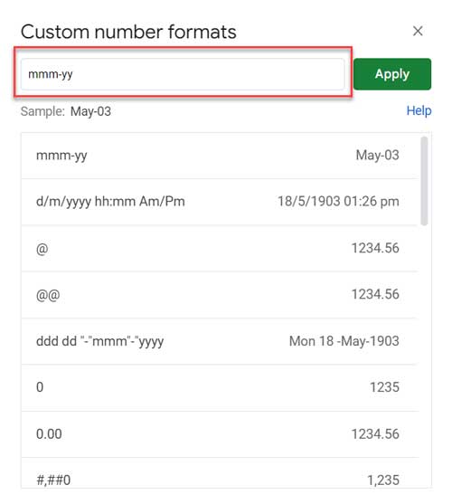
Select B2:B8 and go to the Format menu > Number > Custom number format and apply the format mmm-yy.
Pivot Table:
Now time to group dates by month using the Pivot table in Google Sheets.
We will group by the newly added month helper column B instead of the date column A.
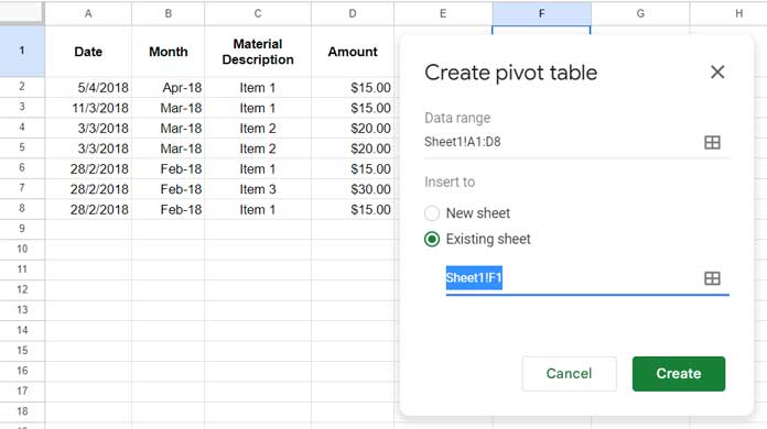
1. Select the range A2:D8.
2. Go to the Insert menu > Pivot table.
3. Check “Existing Sheet” and cell F1 to create the month-wise Pivot table report in the existing Sheet. Of course, you can choose the Sheet and cell to insert the Pivot table in your Sheet.
4. Click Create.
5. On the sidebar panel, “Add” or drag and drop “Month” under the Rows field, “Material Description” under the Columns field, and “Amount” under the Values field, and voila!
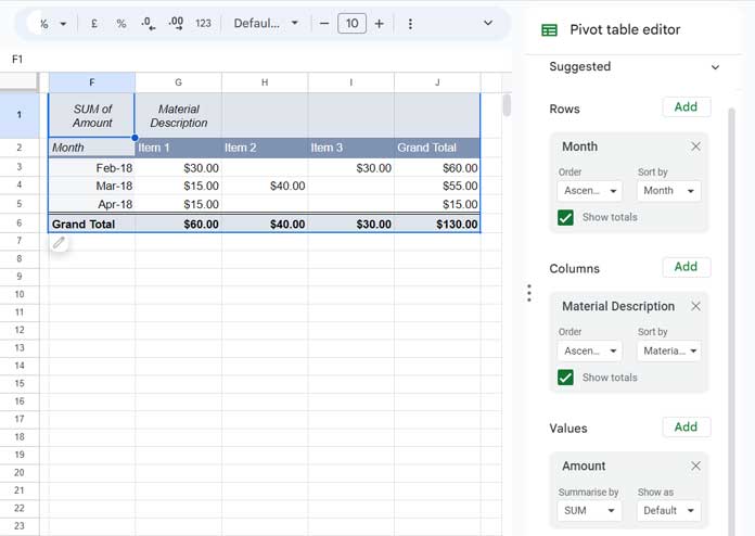
This way we can group dates by month using a Pivot table in Google Sheets.
Note:- If you don’t want the “Material Description” column in the result, do not add it under the “Columns” field.
2. Group Dates by Month in Pivot Table in Google Sheets: New Approach
It is the recommended approach as it doesn’t require a helper column.
Here are the steps to group dates by month in the Pivot table report without a helper column in Google Sheets.
1. Select the range A2:C8 (the ‘original’ data without a helper column inserted).
2. Go to the Insert menu > Pivot table.
3. Check “Existing Sheet” and cell F1 (if you want, you can choose a different Sheet and cell).
4. Click Create.
5. On the sidebar panel, “Add” or drag and drop “Date” under the Rows field, “Material Description” under the Columns field, and “Amount” under the Values field.
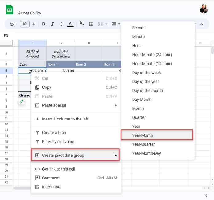
6. Right-click on any date in the first column in the Pivot table report and select Create pivot date group > Year-Month, and voila!
Month-Wise Pivot Table Using Query Formula in Google Sheets
This section is for enthusiasts in Google Sheets functions.
If you are new to Query, please check my Google Sheets Query function step-by-step guide. It has everything for a beginner to learn this most powerful function in Google Sheets.
Let’s see, step by step, how to code a Query formula that can create a month-wise Pivot Table Report in Google Sheets using the date column.
Steps
We can use the MONTH scalar function in Query to group data by month numbers. To group by month name, we will follow a workaround.
We will use a helper column. So we will use the sample data under the title “1. Group Dates by Month in Pivot Table in Google Sheets: Old-School Approach.”
Note:- We can avoid using the helper column. But that may make the formula complex.
We require three Query formulas (in a nested form) to generate the month-wise Pivot table report in Google Sheets.
First, we will use a Query formula to return a month-wise Pivot table report.
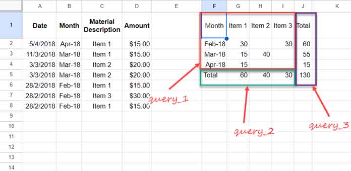
query_1: Group by “Month” and pivot “Material Description.”
=query(A1:D,"Select B,sum(D) where A is not null group by B Pivot C",1)To add a total row at the bottom of the query_1 result, we will require one additional formula, and here it is.
query_2: Group by “Material Description” to return the material-description-wise total. The result is transposed to make it a row.
=transpose(query(A1:D,"Select sum(D) where A is not null group by C label sum(D)'Total'",1))query_3: Group by “Month” to return its month-wise total. To it, vertically appended the sum of the month column.
=vstack(query(A1:D,"Select sum(D) where A is not null group by B label sum(D)'Total'",1),sum(D:D))Let’s use the VSTACK and HSTACK functions to append the above three outputs vertically and horizontally.
Syntax: hstack(vstack(query_1,query_2),query_3)
=hstack(vstack(query(A1:D,"Select B,sum(D) where A is not null group by B Pivot C",1),transpose(query(A1:D,"Select sum(D) where A is not null group by C label sum(D)'Total'",1))),vstack(query(A1:D,"Select sum(D) where A is not null group by B label sum(D)'Total'",1),sum(D:D)))That’s all. Thanks for the stay. Enjoy!
Quick question.
How do I get my pivot table to display or sort my data by month? IE I had no problem making the table but as you can see in the example when I sort by month it sorts alphabetically by the name of the month.
I would like it to sort in chronological order (Jan, Feb, Mar, Apr, etc… ) so that I can look at my year in a glance and easily see my most recent months.
I am using the pivot table method in google sheets.
Thanks!
Hi, Stacey,
Please see this new post. You can group data in month wise (in chronological order) without a helper column.
Month, Quarter, Year Wise Grouping in Pivot Table in Google Sheets