The VSTACK function appends two or more ranges vertically and returns a larger array. It has become one of the most commonly used functions in Google Sheets. You can see its application in both simple formulas and more complex LAMBDA functions, such as REDUCE.
When using the VSTACK function in Google Sheets, you may encounter #N/A errors, blank cells, or blank rows in the output.
In this Google Sheets tutorial, you’ll learn how to use the VSTACK function and how to handle errors or remove blank rows from the output.
Why Use VSTACK Function Instead of Curly Braces?
Another option for stacking data vertically is using curly braces {}. While effective, curly braces come with some limitations. Instead of focusing on these limitations, we’ll highlight the advantages of using VSTACK over curly braces:
- Readability: The VSTACK function makes formulas easier to read, especially when working with large datasets.
- No need for semicolons: With VSTACK, you can use the standard argument separator (commas or semicolons, depending on your locale), unlike curly braces where semicolons are required to separate arrays.
- Handling different-sized arrays: If the arrays have different widths, curly braces return a #VALUE! error, whereas VSTACK can handle arrays with varying numbers of columns (though it may return #N/A errors for missing values).
VSTACK Function: Syntax and Arguments
Syntax:
VSTACK(range1, [range2, …])Arguments:
- range1: The first array or range to append.
- range2, …: Additional arrays or ranges (optional) to append vertically below the first range.
Basic Formula Examples
Here’s a simple example of stacking two equal-sized ranges:
=VSTACK(Sheet1!A2:C10, Sheet2!A2:C10)In the following example, the first range contains two columns, and the second range contains three columns:
=VSTACK(B3:C5, E3:G5)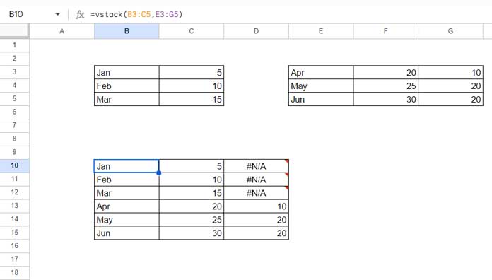
In this case, VSTACK automatically adjusts to return the maximum number of columns between the two ranges. However, it fills the extra columns with #N/A errors when the number of columns doesn’t match. How can we remove these errors?
Removing #N/A Errors in VSTACK
Since VSTACK doesn’t have a pad_with argument (unlike the WRAPCOLS or WRAPROWS functions), we need to use the IFNA function to replace #N/A with a value like 0, a blank, or any other desired value.
Here’s how to replace #N/A with 0:
=IFNA(VSTACK(B3:C5, E3:G5), 0)Handling Blank Rows in VSTACK
A common issue arises when stacking multiple QUERY results with VSTACK—you might end up with blank rows or rows full of #N/A values between the results. This happens when one or more QUERY formulas return no matching results.
Example (Formula in cell B9):
=VSTACK(
   QUERY(B2:C6, "SELECT * WHERE Col1 = 'a'"),
   QUERY(E2:F6, "SELECT * WHERE Col1 = 'b'"),
   QUERY(H2:I6, "SELECT * WHERE Col1 = 'c'")
)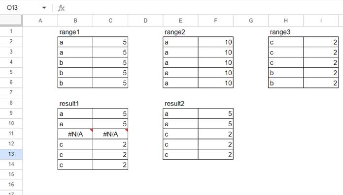
If the second QUERY returns no results (i.e., no rows where Col1 = ‘b’), VSTACK leaves a row of #N/A values.
To replace #N/A with blanks, you can use IFNA:
=IFNA(
   VSTACK(
      QUERY(B2:C6, "SELECT * WHERE Col1 = 'a'"),
      QUERY(E2:F6, "SELECT * WHERE Col1 = 'b'"),
      QUERY(H2:I6, "SELECT * WHERE Col1 = 'c'")
   )
)
But this can still leave a blank row. How do we remove such blank rows?
Removing Blank Rows in VSTACK
We can use the LET function to define the VSTACK result and then filter out the blank rows.
=LET(
   result,
   IFNA(
      VSTACK(
         QUERY(B2:C6, "SELECT * WHERE Col1 = 'a'"),
         QUERY(E2:F6, "SELECT * WHERE Col1 = 'b'"),
         QUERY(H2:I6, "SELECT * WHERE Col1 = 'c'")
      )
   ),
   FILTER(result, INDEX(result, 0, 1) <> "")
)
VSTACK Function with REDUCE Function
This section uses the LAMBDA function and is intended for advanced users.
The REDUCE function applies a LAMBDA function to an array, reducing it row by row while storing intermediate values in an accumulator. If you want to keep track of these intermediate values, you can use VSTACK to “stack” the accumulator value after each iteration.
Example:
Assume we have a list of items in A2:A. First, we extract unique items from this list:
=UNIQUE(A2:A)Now, let’s use REDUCE to apply a LAMBDA function to these unique values and stack the results using VSTACK:
=REDUCE(TOCOL(,1), B2:B4, LAMBDA(acc, val, VSTACK(acc, FILTER(A2:A, A2:A = val),"*")))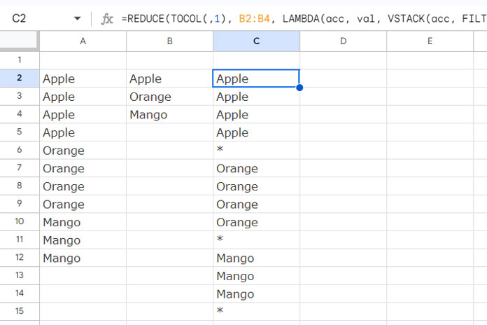
In this formula:
- REDUCE iterates over each value in B2:B4.
- For each value, it filters the range A2:A to match the current value (val).
- VSTACK then stacks the accumulator (acc) with the filtered result, placing a
"*"between each filtered result for clarity.
This method allows us to progressively accumulate and display the results, with each iteration adding new filtered results and a separator (“”) between them.
Conclusion
The VSTACK function is a powerful tool for appending data vertically in Google Sheets, offering better flexibility and readability than curly braces. By combining it with functions like IFNA, IFERROR, and LET, you can handle errors and blank rows more effectively.


