The WRAPCOLS function in Google Sheets is a powerful array function designed to transform a single row or column into multiple columns. It simplifies the process of reshaping data into a two-dimensional array format.

While we can use a combination of OFFSET, QUERY, or even VLOOKUP with SEQUENCE to achieve similar results, most of these methods are more complex. The WRAPCOLS function offers a straightforward and efficient solution.

In a recent tutorial, I also introduced its counterpart, WRAPROWS. But how do these two functions differ in functionality?

• WRAPCOLS arranges data in columns.
• WRAPROWS arranges data in rows.

WRAPCOLS Function: Syntax and Arguments

Syntax:

WRAPCOLS(range, wrap_count, [pad_with])

Arguments:

• range: The array or range of values to wrap. This range can be either a single row or a single column.
• wrap_count: The maximum number of values for each column in the output. If this value isn’t a whole number (e.g., 5.5), the function rounds it down to the nearest integer.
• pad_with: (Optional) A value to replace #N/A in blank cells when the data doesn’t perfectly fit into the specified columns.

Example of WRAPCOLS Function Usage

Consider the following example: Q1, Q2, Q3, and Q4 month-wise sales values are listed in a column under corresponding labels. You want to transform this data into separate columns for each quarter.

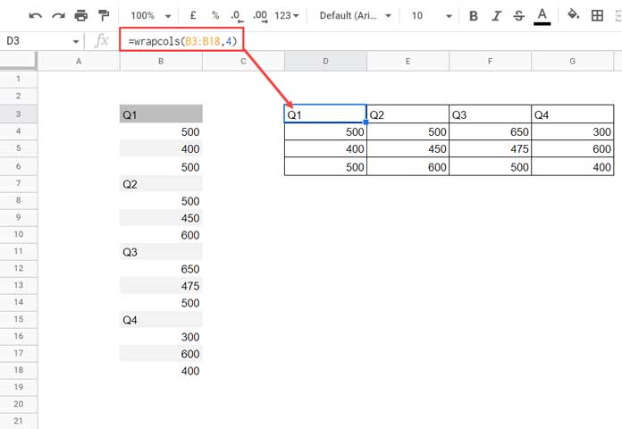
Here’s the WRAPCOLS formula I used in cell D3:

=WRAPCOLS(B3:B18, 4)

In this example:

• The range is B3:B18, containing the sales data.
• The wrap_count is 4, which means the data will be wrapped into four columns.

This is a more efficient approach compared to older methods. Previously, I might have used the following formula as an alternative:

=ARRAYFORMULA(VLOOKUP(TRANSPOSE(SEQUENCE(4, 4, ROW(B3))), {ROW(B3:B18), B3:B18}, 2, 0))

This combination of SEQUENCE, VLOOKUP, and ARRAYFORMULA can achieve similar results, but it’s more complex and less intuitive than using WRAPCOLS.

Using the pad_with Argument

The pad_with argument can be used to handle missing data. For example:

=WRAPCOLS(A1:A5, 3)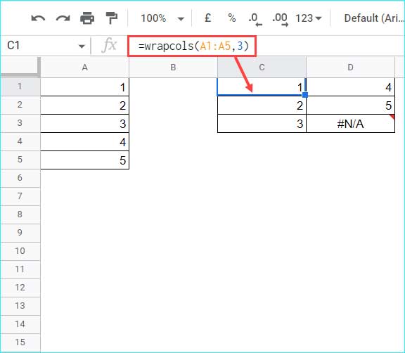

In this case, the range A1:A5 contains five elements, but the wrap_count is 3. This means the last cell in the second column will be blank, and by default, the function will return #N/A.

To replace #N/A with a custom value, such as “no value,” use the pad_with argument like this:

=WRAPCOLS(A1:A5, 3, "no value")

Sorting Data in a Two-Dimensional Array

Let’s now explore how to use the WRAPCOLS function as part of sorting a 2D array.

Imagine we have monthly sales data for Q1, Q2, Q3, and Q4 in the range D3:G6.

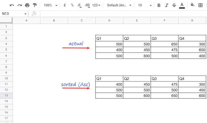
How can we sort the values within each quarter in ascending or descending order? And what role does the WRAPCOLS function play in this process?

Sorting in Ascending Order

To sort the sales data for each quarter, we’ll break the formula down step by step:

Copy the field labels (Q1, Q2, Q3, Q4) from cells D3:G3 and paste them into D10:G10.

We have a 3×4 matrix (3 rows and 4 columns) of sales data, excluding the header. Use the following MAKEARRAY formula in cell D11 to generate a matrix of similar dimensions:

=MAKEARRAY(3, 4, LAMBDA(r, c, c + 0))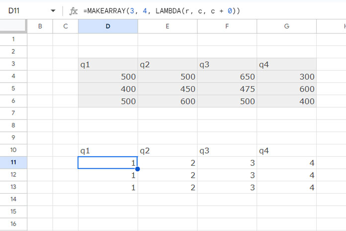

Flatten this array to convert it into a single column:

=FLATTEN(MAKEARRAY(3, 4, LAMBDA(r, c, c + 0)))

Next, flatten the actual sales data (excluding the labels):

=FLATTEN(D4:G6)

Combine the two flattened arrays into a two-column array:

={FLATTEN(MAKEARRAY(3, 4, LAMBDA(r, c, c + 0))), FLATTEN(D4:G6)}

Sort the array in ascending order, first by the first column, then by the second column:

=SORT(
   {FLATTEN(MAKEARRAY(3, 4, LAMBDA(r, c, c + 0))), FLATTEN(D4:G6)}, 
   1, 1, 2, 1
)

Extract the sorted sales figures (second column) using INDEX:

=INDEX(
   SORT(
      {FLATTEN(MAKEARRAY(3, 4, LAMBDA(r, c, c + 0))), FLATTEN(D4:G6)}, 
      1, 1, 2, 1
   ), 0, 2
)

Finally, wrap the sorted data back into a two-dimensional array using WRAPCOLS:

=WRAPCOLS(
   INDEX(
      SORT(
         {FLATTEN(MAKEARRAY(3, 4, LAMBDA(r, c, c + 0))), FLATTEN(D4:G6)}, 
         1, 1, 2, 1
      ), 0, 2
   ), 3
)

This formula arranges the sorted sales values into a 3×4 matrix.

Sorting in Descending Order

To sort the sales values in descending order, you only need to modify one parameter in the SORT function:

Change the last 1 to 0 to sort the second column (sales figures) in descending order:

=WRAPCOLS(
   INDEX(
      SORT(
         {FLATTEN(MAKEARRAY(3, 4, LAMBDA(r, c, c + 0))), FLATTEN(D4:G6)}, 
         1, 1, 2, 0
       ), 0, 2
   ), 3
)

And that’s how you can use the WRAPCOLS function in Google Sheets to wrap data, handle missing values, and sort two-dimensional arrays efficiently.

Thank you for reading! Enjoy exploring the WRAPCOLS function in your sheets.