Need a fair formula to split fuel costs among travelers on a long road trip?
Splitting a gas bill equally isn’t fair if one passenger hops out after 50 kilometers while another stays for the whole 500-kilometer journey. To handle this properly, you must calculate the cost per kilometer, track individual travel segments, and divide the cost of each leg only among the passengers who were actually in the vehicle.
In this tutorial, you’ll learn how to use a single Google Sheets dynamic array formula to automate this entire process using odometer entries.
💡 Prefer a ready-made solution? If you want to skip the formula-building process and download a pre-configured dashboard, check out my guide: Road Trip Fuel Cost Splitter in Google Sheets (Free Template).
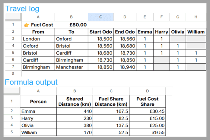
1. Arrange the Travel Log (Sheet1)
To ensure the formula maps ranges accurately without throwing #REF! or #VALUE! errors, your data structure must match the exact row configuration below. Place your total fuel cost in cell B1, your field labels in Row 2, and begin your actual travel log data inputs on Row 3.
| A | B | C | D | E | F | G | H | |
| 1 | Total Fuel Cost: | 150.00 | ||||||
| 2 | From | To | Start Odo | End Odo | Emma | Harry | Olivia | William |
| 3 | London | Oxford | 18,500 | 18,560 | 1 | 1 | ||
| 4 | Oxford | Bristol | 18,560 | 18,680 | 1 | 1 | 1 | |
| 5 | Bristol | Cardiff | 18,680 | 18,730 | 1 | 1 | 1 | 1 |
| 6 | Cardiff | Birmingham | 18,730 | 18,850 | 1 | 1 | 1 | |
| 7 | Birmingham | Manchester | 18,850 | 18,940 | 1 | 1 |
Data Entry Ground Rules
- Row 2 (Field Labels): Passenger names must begin exactly in column E (
E2:H2). - Row 3 Down (Input Data): Enter 1 under each passenger who was present during that specific leg. Leave the cell completely blank if they were not in the vehicle.
- Continuous Mileage: The ending odometer reading of one segment must match the starting odometer reading of the next segment.
2. The Fuel Cost Split Formula (Sheet2)
Create a second sheet tab named Sheet2. Select cell A1 and paste the master formula below. Ensure the cells below and to the right of A1 are empty so the dynamic array has room to expand.
=ArrayFormula(LET(
  expn, Sheet1!B1,
  startOdo, Sheet1!C3:C,
  endOdo, Sheet1!D3:D,
  status, Sheet1!E3:H,
  headers, Sheet1!E2:H2,

  sharedDist, endOdo - startOdo,
  peopleCount, BYROW(status, LAMBDA(r, SUM(r))),

  fuelShareDist, IFERROR(sharedDist / peopleCount),

  costPerKm, expn / SUM(sharedDist),

  colSum, LAMBDA(data, BYCOL(status, LAMBDA(c, SUMPRODUCT(c * data)))),

  sharedSummary, colSum(sharedDist),
  fuelShareSummary, colSum(fuelShareDist),
  costSummary, fuelShareSummary * costPerKm,

  summary,
    VSTACK(headers, sharedSummary, fuelShareSummary, costSummary),

  final,
    VSTACK(
      HSTACK("Person","Shared Distance (km)","Fuel Share Distance (km)","Fuel Cost Share"),
      TRANSPOSE(FILTER(summary, INDEX(summary,4,0)>0))
    ),

  IFNA(final)
))
The formula will automatically compile the names, aggregate individual distances, apply the per-kilometer cost weight, and return a clean, 4-column summary grid.
3. How the Formula Works (Variable Logic Breakdown)
By leveraging the LET function, this multi-step mathematical problem is broken down into highly readable logic variables:
| Variable | Structural Formula / Logic | What It Calculates |
sharedDist | endOdo - startOdo | Determines the total distance covered during an isolated leg of the trip. |
peopleCount | BYROW(status, LAMBDA(r, SUM(r))) | Scans each row individually to count how many occupants are splitting the cost for that specific leg. |
fuelShareDist | IFERROR(sharedDist / peopleCount) | Allocates proportional distance responsibility per leg (prevents #DIV/0! errors if a row is left blank). |
costPerKm | expn / SUM(sharedDist) | Calculates the precise financial weight of a single kilometer based on your total fuel cost in B1. |
colSum | LAMBDA(data, BYCOL(status, …)) | A reusable temporary function that loops through each passenger column and aggregates calculations, eliminating the need to write duplicate loops. |
Hiding Empty/Zero-Cost Passengers
The final step uses INDEX(summary, 4, 0) > 0 inside a FILTER function.
Because summary stacks our calculated totals vertically, row 4 represents the calculated costSummary. If a passenger is listed in your header row labels (E2:H2) but never actually checked into any leg of the trip, this filter automatically excludes them from the final summary output grid instead of cluttering your spreadsheet with zero-value rows.
Conclusion
This advanced Google Sheets formula provides a fair, automated way to allocate travel expenses when passengers join or leave a vehicle during different points of a journey. By combining LET, BYROW, BYCOL, and SUMPRODUCT, you remove the tedious manual math from vacation planning.


