Conquer Duplicate IDs: Master Left, Right, Inner, & Full Joins in Google Sheets

Basic Joins in Google Sheets, such as left, right, inner, or full, assume one table has unique IDs, while the other may or may not. We’ve covered this before. But what if neither table, one table, or both have duplicates?

Introducing a powerful combination of REDUCE, FILTER, and OFFSET (with additional functions to unlock its full potential)! This formula handles any scenario: one table with duplicates, both tables with duplicates, or neither.

Master left, right, inner, and full joins without worrying about duplicates! This isn’t just joining; it’s a skill-boosting adventure with never-before-seen Google Sheets tricks.

Prerequisites:

The unique ID column must be the first column in both tables.
Physical data ranges (not formulas).

While the core formula for all joins (with or without duplicates) remains consistent, slight adjustments are needed depending on the join type. Full joins have an extra step, but the first three types share similar modifications.

Conquering Duplicate IDs: Sample Data for All Join Types in Google Sheets

Duplicate IDs wreaking havoc in your Google Sheets joins? Fear not! This tutorial equips you with “all-weather” formulas to conquer Left, Right, Inner, and Full Joins, even with duplicate IDs in your unique identifier column.

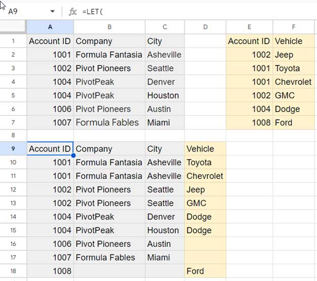
Our example involves two tables: Customer Data (with columns for Account ID, Company, and City) and Vehicle Information (with columns for Account ID and Model).

Left Table: Customer Data

Account ID	Company	City
1001	Formula Fantasia	Asheville
1002	Pivot Pioneers	Seattle
1004	PivotPeak	Denver
1004	PivotPeak	Houston
1006	Pivot Pioneers	Austin
1007	Formula Fables	Miami

Right Table: Vehicle Information

Account ID	Vehicle
1002	Jeep
1001	Toyota
1001	Chevrolet
1002	GMC
1004	Dodge
1008	Ford

Both tables contain duplicates in the unique identifier column (Account ID).

In the first table, some companies appear in multiple cities, reflecting branch locations or overlapping territories. Meanwhile, the second table reveals instances where a single company owns several vehicles.

Adding to the complexity, some Account IDs exist in one table but not the other, further challenging traditional join methods.

Mastered joins without duplicate IDs? Check out our tutorials on:

Left Joins: How to Left Join Two Tables in Google Sheets
Right Joins: How to Right Join Two Tables in Google Sheets
Inner Joins: How to Inner Join Two Tables in Google Sheets
Full Joins: How to Full Join Two Tables in Google Sheets

Unlike the formulas presented in my previous ‘join’ tutorials, the formulas in this tutorial require physical tables, and the ID column must be the first column in both tables. This adjustment ensures compatibility with scenarios involving duplicate IDs.

However, the formulas provided here are versatile and can be used confidently for all join types in Google Sheets. They are designed to handle various situations, making them reliable solutions for your data joining needs.

Click the button below to copy my sample sheet with examples and formulas.

Sample Sheet

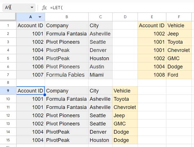
Handling Duplicate IDs in Left Joins on Source Tables

A left join combines all records from the left table with the matching records from the right table.

As I mentioned at the beginning of this tutorial, here we will use a powerful key combination of REDUCE, FILTER, and OFFSET for a left join without worrying about duplicate IDs in the tables.

Formula:

=LET(
   lt_id_field, A1:A7, 
   lt_range, A1:C7, 
   rt_id_field, E1:E7, 
   rt_range_x_id, F1:F7, 
   merge, 
   REDUCE("", lt_id_field, LAMBDA(a, v, VSTACK(a, IFNA(
      HSTACK(
         OFFSET(v, 0, 0, 1, COLUMNS(lt_range)), 
         FILTER(rt_range_x_id, rt_id_field=v)
      ), OFFSET(v, 0, 0, 1, COLUMNS(lt_range)))))
   ), 
   IFNA(FILTER(merge, CHOOSECOLS(merge, 1)<>""))
)

Result:

Left Join with Duplicate IDs in Both Tables in Google Sheets

How do I use this formula?

You can utilize this formula by adjusting the range references as explained in the table below:

Name	Range	Description
lt_id_field	A1:A7	Left table ID column
lt_range	A1:C7	Left table range (including ID and other data)
rt_id_field	E1:E7	Right table ID column
rt_range_x_id	F1:F7	Right table range excluding the ID field

Replace the ranges A:A7, A1:C7, E1:E7, and F1:F7 in the formula with the corresponding ranges in your table. No other changes are required.

Explanation:

LET function: Assigns names to ranges and intermediate calculations for easier reference and formula modification.
REDUCE and LAMBDA: Loop through each ID in the left table.
HSTACK, OFFSET, and FILTER: For each ID, combine the left table row with matching right table rows (even if multiple).
IFNA: Handle potential missing values.
CHOOSECOLS and FILTER: Extract the final result, excluding the first empty row.

Formula Break-Down

We have observed the range references in the formula and their corresponding names. Additionally, we have used another name, ‘merge,’ for the intermediate formula, which is as follows:

REDUCE("", lt_id_field, LAMBDA(a, v, VSTACK(a, IFNA(HSTACK(OFFSET(v, 0, 0, 1, COLUMNS(lt_range)), FILTER(rt_range_x_id, rt_id_field=v)),OFFSET(v, 0, 0, 1, COLUMNS(lt_range))))))

Let’s delve into this part in detail, as it is the core of left joining two tables without worrying about duplicate IDs in Google Sheets.

Part 1: Handling Duplicate IDs

HSTACK(OFFSET(v, 0, 0, 1, COLUMNS(lt_range)), FILTER(rt_range_x_id, rt_id_field=v))

We can interpret it as:

HSTACK(OFFSET(v, 0, 0, 1, COLUMNS(A1:C7)), FILTER(F1:F7, E1:E7=v))

This part focuses on dealing with duplicate IDs in the join operation. Let’s break it down:

HSTACK: This function horizontally stacks arrays on top of each other. It’s used to combine the relevant rows from both tables.

OFFSET(v, 0, 0, 1, COLUMNS(lt_range)): This part retrieves the entire row containing the current element (v) from the left table (lt_range).
- v: This refers to the current element in the array during the REDUCE function (e.g., A1 in the first row, A2 in the second, etc.).
- 0, 0: These specify no offset from the current cell (v).
- 1: This indicates returning the entire row containing v, regardless of the actual number of columns.
- COLUMNS(lt_range): This dynamically retrieves the number of columns in the left table range and sets the width of the returned array.

FILTER(rt_range_x_id, rt_id_field=v): This filters the right table (rt_range_x_id) based on the current element (v). It selects rows where the value in the right table’s ID field (rt_id_field) matches the current element (v).
- It selects rows from the right table based on the current element’s ID value, ensuring matching records are combined.

Interpretation:

This part essentially combines two elements:

The entire row contains the current element from the left table.
All matching rows from the right table where the ID field values match the current element.

Part 2: Duplicating a Left Table Record

IFNA(part_1, OFFSET(v, 0, 0, 1, COLUMNS(lt_range))

We can interpret it as:

IFNA(part_1, OFFSET(v, 0, 0, 1, COLUMNS(A1:C7))

This part addresses cases where FILTER in Part 1 returns multiple rows in the right table for a single element (v) in the left table.

For example, imagine element v has two matching rows in the right table. The current formula would combine the single left table row with all two right table rows horizontally, leading to #N/A in some columns due to mismatched row sizes.

Example:

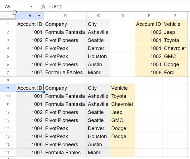
1001	Formula Fantasia	Asheville	Toyota
#N/A	#N/A	#N/A	Chevrolet

Note: Check out the screenshot below to see Account ID 1001 in both tables. You’ll notice “Toyota” and “Chevrolet” listed for this ID in the right table, demonstrating how our formulas handle duplicate IDs in joins.

To address this, we use IFNA to replace any #N/A errors with the corresponding entries from the current left table row. This ensures a complete row even if there are multiple matches in the right table.

The IFNA function checks for errors and replaces them with the value provided as the second argument. In this case, we use OFFSET(v, 0, 0, 1, COLUMNS(lt_range)) to retrieve the entire left table row for the current element (v). This ensures the entire left table row is replicated for any #N/A encountered.

Result:

1001	Formula Fantasia	Asheville	Toyota
1001	Formula Fantasia	Asheville	Chevrolet

By using IFNA and OFFSET, we effectively handle situations with multiple right table matches, filling in missing values with the corresponding entries from the left table row.

We need to use another IFNA to address potential errors related to missing matching rows in the right table. This will be utilized in the formula_expression below.

REDUCE and LAMBDA Part:

The REDUCE function, a LAMBDA helper function, iterates over each element (v) in the left table’s Account ID array, accumulating all matched rows from the right table for each unique ID.

It starts with an empty string ("") as the accumulator (a). The LAMBDA function takes this accumulator and the current element (v) as arguments. Inside the LAMBDA:

part_2 is calculated, which combines the left table row with the matching right table rows and uses IFNA to replace #N/A with the corresponding left table entries.
This calculated result from part_2 is then vertically stacked (VSTACK) onto the existing accumulator (a).

By iterating over each element and accumulating the results, the REDUCE function builds a final output containing all matched right table rows for each left table ID, even if duplicates exist. This effectively performs a left join, handling duplicate IDs by accumulating separate sets of right table matches for each unique left table ID.

Formula Expression

The IFNA(FILTER(merge, CHOOSECOLS(merge, 1)<>"")) expression performs two actions:

Filtering: It uses FILTER to select rows from the merge array where the value in the first column (identified by CHOOSECOLS(merge, 1)) is not an empty string. This excludes any rows with no data in the first column.
Handling errors: It wraps the FILTER function in IFNA to handle potential errors, such as if the merge is empty. In case of errors, IFNA would return an empty string.

Handling Duplicate IDs in Right Joins on Source Tables

A right join combines all records from the right table with the matching records from the left table.

I have provided a detailed explanation of the left join formula that handles duplicate IDs.

You can use that formula for a right join with a few changes in the range references and assigned names for the right join.

In the left join, we used the following names and range references:

lt_id_field, A1:A7
lt_range, A1:C7
rt_id_field, E1:E7
rt_range_x_id, F1:F7

When it comes to the right join, you should use the following names and range references:

rt_id_field, E1:E7
rt_range, E1:F7
lt_id_field, A1:A7
lt_range_x_id, B1:C7

This is because we need to FILTER the left table, and the REDUCE operation is applied to the right table. So, in the formula, you should use the range names accordingly.

Formula:

=LET(
   rt_id_field, E1:E7, 
   rt_range, E1:F7, 
   lt_id_field, A1:A7, 
   lt_range_x_id, B1:C7, 
   merge, 
   REDUCE("", rt_id_field, LAMBDA(a, v, VSTACK(a, IFNA(
      HSTACK(
         OFFSET(v, 0, 0, 1, COLUMNS(rt_range)), 
         FILTER(lt_range_x_id, lt_id_field=v)
      ), OFFSET(v, 0, 0, 1, COLUMNS(rt_range)))))
   ), 
   IFNA(FILTER(merge, CHOOSECOLS(merge, 1)<>""))
)

Result:

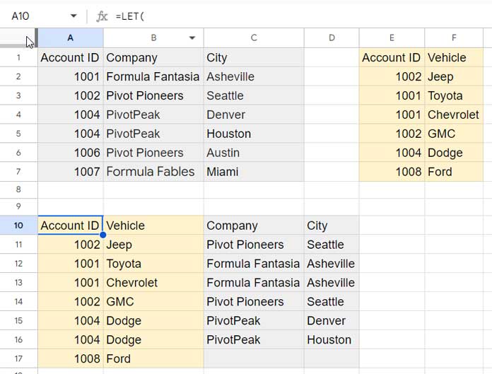
Right Join with Duplicate IDs in Both Tables in Google Sheets

You can use this formula to right-join two tables without worrying about duplicate IDs in the unique identifier fields.

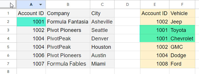
Handling Duplicate IDs in Inner Joins on Source Tables

An inner join combines only the matching records from both tables.

For an inner join, you can use the left join or right join formula with a minor change in the formula_expression part.

The formula expression part is originally IFNA(FILTER(merge, CHOOSECOLS(merge, 1)<>"")). To adapt it for an inner join, replace it with IFNA(FILTER(merge, CHOOSECOLS(merge, -1)<>"")).

In left and right joins, the formula expression is used to filter out blank rows if the first column in the ‘merge’ is blank.

This essentially removes a blank row added during REDUCE at the top.

In the left or right join, if any cell in the last column is blank, it means it’s either the blank row returned by the REDUCE or a mismatching row in either of the tables.

If you need the formula, here is the left join formula converted to an inner join:

=LET(
   lt_id_field, A1:A7, 
   lt_range, A1:C7, 
   rt_id_field, E1:E7, 
   rt_range_x_id, F1:F7, 
   merge, 
   REDUCE("", lt_id_field, LAMBDA(a, v, VSTACK(a, IFNA(
      HSTACK(
         OFFSET(v, 0, 0, 1, COLUMNS(lt_range)), 
         FILTER(rt_range_x_id, rt_id_field=v)
      ), OFFSET(v, 0, 0, 1, COLUMNS(lt_range)))))
   ), 
   IFNA(FILTER(merge, CHOOSECOLS(merge, -1)<>""))
)

Result:

Inner Join with Duplicate IDs in Both Tables in Google Sheets

This formula joins the two tables if both tables match the Account ID. Duplicate Account IDs will also be matched and returned.

Handling Duplicate IDs in Full Joins on Source Tables

A full join combines all records from both tables.

For a full join, you can use the left join formula. However, unlike right and inner joins, an additional step is required. I’ll explain why this step is necessary.

The left join returns all records from the left table and only the matching records from the right table. To include the mismatching records from the right table, an additional step is needed.

Here is the formula piece that you need to vertically join with the left join formula:

=IFERROR(
   FILTER(
      HSTACK(E1:E7, SEQUENCE(1, COLUMNS(A1:C7)-1)/0, F1:F7), 
      IFNA(XMATCH(E1:E7, A1:A7))=""
   )
)

Explanation

To filter the mismatching records from the right table, the right table range is E1:F7. However, the range used in the FILTER is as follows:

HSTACK(E1:E7, SEQUENCE(1, COLUMNS(A1:C7)-1)/0, F1:F7)

This accommodates the table structure of the left join result:

The left table contains three columns.
The right table contains two columns.

The left join returns 3+2-1, i.e., 4 columns. We deduct 1 column as the formula removes multiple occurrences of the Account ID column.

Using the range E1:F7 directly won’t append the filtered range correctly with the left join result, as it won’t match columns.

Therefore, we stack the right table ID column, columns with errors matching the number of columns in the left table, plus the right table columns excluding the ID column. This ensures the number of columns in the above filter formula matches the number of columns in the left join formula.

How does the FILTER filter the rows containing Account IDs that are not available in the left table?

The FILTER filters the above range if IFNA(XMATCH(E1:E7, A1:A7))="".

The XMATCH matches the right table IDs in the left table and returns the matching position or #N/A. The IFNA converts errors to blanks, and the FILTER filters those blank rows.

Finally, the IFERROR removes error values.

Converting Left Join Formula to Full Join

We can concatenate the formulas as follows:

=VSTACK(left_join_formula, filter_formula)

However, this approach won’t be dynamic. To maintain consistency with the assigned names for ranges in FILTER, we can incorporate the FILTER within the left join formula. This enables us to use the same assigned names for ranges in FILTER.

What we need to do is insert one more intermediate calculation (the aforementioned filter formula) after the merge. We can name it missing and vertically stack it in the formula expression.

Formula:

=LET(
   lt_id_field, A1:A7, 
   lt_range, A1:C7, 
   rt_id_field, E1:E7, 
   rt_range_x_id, F1:F7, 
   merge, 
   REDUCE("", lt_id_field, LAMBDA(a, v, VSTACK(a, IFNA(
      HSTACK(
         OFFSET(v, 0, 0, 1, COLUMNS(lt_range)), 
         FILTER(rt_range_x_id, rt_id_field=v)
      ), OFFSET(v, 0, 0, 1, COLUMNS(lt_range)))))
   ), 
   missing, 
      IFERROR(FILTER(
         HSTACK(rt_id_field, SEQUENCE(1, COLUMNS(lt_range)-1)/0, rt_range_x_id), 
         IFNA(XMATCH(rt_id_field, lt_id_field))=""
      )),
   VSTACK(IFNA(FILTER(merge, CHOOSECOLS(merge, 1)<>"")), missing)
)

Result:

Full Join with Duplicate IDs in Both Tables in Google Sheets

Additional Notes

All the provided formulas are flexible and easily adaptable to your data ranges, even for beginners. However, from a learning perspective, understanding the formula structure may require careful attention and could be intimidating for novice users.

The formula utilizes REDUCE and OFFSET, with the former being a lambda helper function and the latter a volatile function. Consequently, you may experience performance issues when working with large datasets. Nevertheless, I have avoided nested lambdas to enhance performance.

In the processed data, if you wish to eliminate duplicate records, consider using the UNIQUE function. For removing duplicates based on any column, the SORTN function can be employed.

Similarly to most formulas, if your data contains a date column, the resulting table may display a date value column instead. You can revert it to the date format using the Format > Number > Date command.

For merging tables using QUERY, please check out this resource: Merge Two Tables in Google Sheets – The Ultimate Guide.