To left join two tables in Google Sheets, you can use an array formula. Though the formula may seem complex, customizing it for your specific table ranges is a simple task.
The LET function is utilized to assign names to expressions. You will need to specify the table ranges and ID columns in both tables, and the formula will take care of the rest.
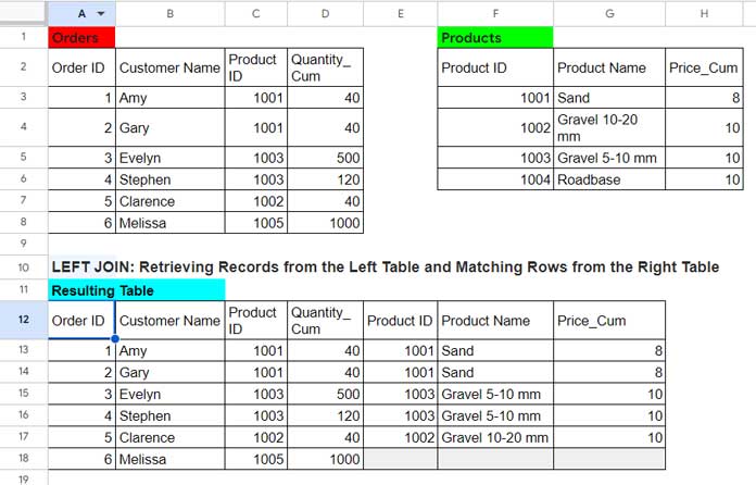
In a left join, two tables are combined into a new one, retaining all rows from the first table (left table) and incorporating matching rows from the second table (right table) based on a shared field (e.g., ID).
A crucial prerequisite for left joining two tables is a shared field in both tables, such as IDs (e.g., employee IDs, product IDs).
Note: If you have duplicated IDs in both ID columns (left and right tables), please check out this guide: Conquer Duplicate IDs: Master Left, Right, Inner, & Full Joins in Google Sheets.
Are you prepared to unleash the potential of left joins? Explore the next section for a comprehensive breakdown of the formula and its application!
Left Join Two Tables: Sample Tables and Resulting Table
This type of left join between two tables typically requires only a VLOOKUP formula in Google Sheets. However, we’ll incorporate additional functions to facilitate adaptation to tables of varying sizes.
Table 1: Orders
| Order_ID | Customer_Name | Product_ID | Quantity_Cum |
| 1 | Amy | 1001 | 40 |
| 2 | Gary | 1001 | 40 |
| 3 | Evelyn | 1003 | 500 |
| 4 | Stephen | 1003 | 120 |
| 5 | Clarence | 1002 | 40 |
| 6 | Melissa | 1005 | 1000 |
This table contains 6 records (6 orders) and four columns, and the Product_ID in the third column uniquely identifies each product.
Table 2: Products
| Product ID | Product Name | Price_Cum |
| 1001 | Sand | 8 |
| 1002 | Gravel 10-20 mm | 10 |
| 1003 | Gravel 5-10 mm | 10 |
| 1004 | Roadbase | 10 |
This table contains 4 records (4 products) and three columns, and the Product_ID in the first column uniquely identifies each product. Please note that in this table, the unique identifiers, i.e., Product IDs in the first column, must not be repeated.
Expected Result:
| Order ID | Customer Name | Product ID | Quantity_Cum | Product Name | Price_Cum |
| 1 | Amy | 1001 | 40 | Sand | 8 |
| 2 | Gary | 1001 | 40 | Sand | 8 |
| 3 | Evelyn | 1003 | 500 | Gravel 5-10 mm | 10 |
| 4 | Stephen | 1003 | 120 | Gravel 5-10 mm | 10 |
| 5 | Clarence | 1002 | 40 | Gravel 10-20 mm | 10 |
| 6 | Melissa | 1005 | 1000 | N/A | N/A |
Please scroll down to see the screenshot of the above tables in Google Sheets.
Array Formula for Left Joining Two Tables in Google Sheets
This formula performs a left join between two tables in Google Sheets, retaining all records from the left table. It assumes unique records exist in the right table’s ID column.
Formula:
=ArrayFormula(
     LET(
          lt, A2:D8, lt_id, C2:C8, rt, F2:H6, rt_id, F2:F6,
          look_up, IFNA(VLOOKUP(lt_id, HSTACK(rt_id, rt), SEQUENCE(1, COLUMNS(rt), 2), 0)),
          HSTACK(lt, look_up)
     )
)
You can replace the formula expression, i.e., HSTACK(lt, look_up) in the formula with CHOOSECOLS(HSTACK(lt, look_up), {1, 2, 3, 4, 6, 7}) to select the required columns and also in the order you want.
Here is the syntax of the CHOOSECOLS function:
CHOOSECOLS(array, [col_num1, …])Note: The formula may convert dates to date values. Therefore, if any column in the left or right table contains a date field, the corresponding field in the resulting table must be formatted as a date using Format > Number > Date.
You can find the left join array formula in cell A12 of the second sheet in the provided sample sheet below.
Formula Breakdown
The formula utilizes the LET function to assign ‘name’ to ‘value_expression’ results and returns the result of the ‘formula_expression’, which represents the resulting table from the left join.
Syntax of the LET Function:
LET(name1, value_expression1, [name2, …], [value_expression2, …], formula_expression)LET Assignments:
lt(name1): Defines the data range of the left table, including the header row.A2:D8(value_expression1): Data range of the left table.
lt_id(name2): Defines the ID column of the left table, including the header row.C2:C8(value_expression2): ID column of the left table.
rt(name3): Defines the data range of the right table, including the header row.F2:H6(value_expression3): Data range of the right table.
rt_id(name4): Defines the ID column of the right table, including the header row.F2:F6(value_expression4): ID column of the right table.
Note: You only need to specify the above value_expressions 1 to 4 concerning your tables. The left join array formula will take care of the rest.
Remaining LET Assignments:
look_up(name5):IFNA(VLOOKUP(lt_id, HSTACK(rt_id, rt), SEQUENCE(1, COLUMNS(rt), 2), 0))(value_expression5): VLOOKUP searches for the IDs from the left table (lt_id) within the ID column of the right table (rt_id) and returns matching records from the right table (rt).- HSTACK: Joins the ID column of the right table (
rt_id) with the entire right table data (rt). - SEQUENCE: Generates a range of numbers representing the column positions in the right table (2 to the number of columns as the first column is the stacked
rt_id). - The final argument (0) specifies an exact match.
- The VLOOKUP function returns matching records from the right table for each ID in the left table.
- HSTACK: Joins the ID column of the right table (
Formula_Expression:
HSTACK(lt, look_up): This segment merges the data from the left table (lt) with the lookup result (look_up). However, it’s important to note that the lookup result comprises only the matching records from the right table, not the entire right table. This distinction is crucial as it precisely accomplishes the intended left join functionality.
Conclusion
You now possess a potent tool for left joins in Google Sheets. The merged table can be fine-tuned with QUERY, enabling actions such as column reordering, data sorting, and aggregations.
For further exploration of the QUERY function’s capabilities, you can find numerous tutorials within this blog. These resources will guide you through the syntax and provide practical examples to help you master this versatile function.
Resources:


