We can utilize an array formula in Google Sheets to perform an inner join between two tables based on a common field. This enables the identification of shared information using a common identifier, such as an account number, employee ID, customer ID, or student ID.
An inner join retains only the entries that possess a matching value in the common field across both tables. This is the most commonly used type of table join.
It’s crucial to emphasize that the right table should ideally contain unique values in the common field, signifying that each record in the table is distinct.
Note: If you have duplicated IDs in both ID columns (left and right tables), please check out this guide: Conquer Duplicate IDs: Master Left, Right, Inner, & Full Joins in Google Sheets.
Inner Join Two Tables: Sample Tables and Resulting Table
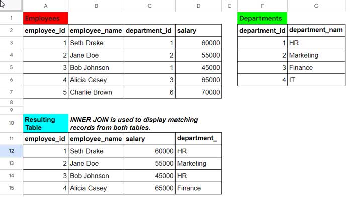
We have two fictitious tables: The left table, ‘Employees,’ includes details about employees, and the right table, ‘Departments,’ contains information about various departments. Our goal is to perform an inner join between these two tables based on the ‘department_id.’ Here are the sample tables and the expected results:
Employees (Left Table):
| employee_id | employee_name | department_id | salary |
| 1 | Seth Drake | 1 | 60000 |
| 2 | Jane Doe | 2 | 55000 |
| 3 | Bob Johnson | 1 | 45000 |
| 4 | Alicia Casey | 3 | 65000 |
| 5 | Charlie Brown | 6 | 70000 |
This table comprises 5 records and 4 columns. The third column, ‘department_id,’ serves as the common field. We aim to match this column in the right table and assign departments.
Departments (Right Table):
| department_id | department_name |
| 1 | HR |
| 2 | Marketing |
| 3 | Finance |
| 4 | IT |
This table contains 4 records and 2 columns. The first column, ‘department_id,’ is the common field.
Please note that the ‘Departments’ table doesn’t contain duplicates in the first column.
Resulting Table (Inner Joined):
| employee_id | employee_name | salary | department_name |
| 1 | Seth Drake | 60000 | HR |
| 2 | Jane Doe | 55000 | Marketing |
| 3 | Bob Johnson | 45000 | HR |
| 4 | Alicia Casey | 65000 | Finance |
The inner joined table contains matching records from both tables based on the ‘department_id’ field.
Array Formula for Inner Joining Two Tables in Google Sheets
The following array formula performs an inner join between two tables in Google Sheets. It assumes unique records in the right table.
Formula:
=ArrayFormula(
     LET(
          lt, A2:D7, lt_id, C2:C7, rt, F2:G6, rt_id, F2:F6,
          look_up, VLOOKUP(lt_id, HSTACK(rt_id, rt), SEQUENCE(1, COLUMNS(rt), 2), 0),
          merge, HSTACK(lt, look_up),
          FILTER(merge, CHOOSECOLS(look_up, 1)<>"")
     )
)
You can wrap the formula expression, i.e., FILTER(merge, CHOOSECOLS(look_up, 1)<>""), in the formula with the CHOOSECOLS function as per the following syntax to select the required columns and also in the order you want.
CHOOSECOLS(array, [col_num1, …])For example, to remove the unique identifiers columns from the inner joined tables, you can replace, FILTER(merge, CHOOSECOLS(look_up, 1)<>"") with CHOOSECOLS(FILTER(merge, CHOOSECOLS(look_up, 1)<>""), {1, 2, 4, 6}).
Note: The inner join formula may convert dates to date values. Therefore, if any column in the left or right table contains a date field, the corresponding field in the resulting table must be formatted as a date using Format > Number > Date.
You can find the inner join array formula in cell A11 of the fourth sheet in the provided sample sheet below.
Formula Breakdown
The above inner join formula in Google Sheets utilizes the LET function to assign ‘name’ to ‘value_expression’ results and returns the result of the ‘formula_expression’, which represents the resulting table from the inner join.
Syntax of the LET Function:
LET(name1, value_expression1, [name2, …], [value_expression2, …], formula_expression)LET Assignments for Inner Join
lt(name1): Defines the data range of the left table (Employees), including the header row.A2:D7(value_expression1): Data range of the left table (Employees).
lt_id(name2): Defines the ID column of the left table (Employees), including the header row.C2:C7(value_expression2): ID column of the left table (Employees).
rt(name3): Defines the data range of the right table (Departments), including the header row.F2:G6(value_expression3): Data range of the right table (Departments).
rt_id(name4): Defines the ID column of the right table (Departments), including the header row.F2:F6(value_expression4): ID column of the right table (Departments).
Note: You only need to specify the value expressions 1 to 4 for your tables. The inner join array formula will take care of the rest.
Remaining LET Assignments for Inner Join
Here, you can understand the logic of inner joining two tables in Google Sheets.
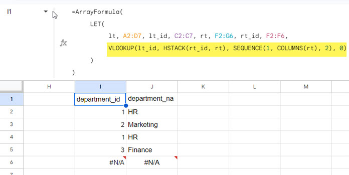
VLOOKUP Part
look_up(name5):VLOOKUP(lt_id, HSTACK(rt_id, rt), SEQUENCE(1, COLUMNS(rt), 2), 0)(value_expression5): This segment of the formula uses VLOOKUP to search for department IDs from the left table within the first column of the stacked arrayHSTACK(rt_id, rt). If a matching ID is found, it retrieves the specified value from the corresponding row in the right table based on the provided sequence of columns. If no matching ID is found, it returns #N/A.
Here’s a breakdown of the components:
- VLOOKUP(lt_id, combined_array, column_indices, 0):
- VLOOKUP searches for each element in the
lt_idarray (department IDs from the left table) within the first column of the combined array created by HSTACK. - The combined array includes the department ID column (
rt_id) as its first column, followed by all columns from the right table (rt). - If a match is found in the first column (department IDs), VLOOKUP then returns the corresponding value from the specified column in the combined array based on the column_indices generated by SEQUENCE.
- VLOOKUP searches for each element in the
- HSTACK(rt_id, rt):
- Joins the department ID column (
rt_id) with the entire right table (rt) horizontally.
- Joins the department ID column (
- SEQUENCE(1, COLUMNS(rt), 2):
- Generates a sequence of numbers starting from 2 and ending at the number of columns in the right table.
- These numbers represent the columns to be returned in the combined array for matching values.
HSTACK Part
merge(name6)HSTACK(lt, look_up)(value_expression6)- This part merges the data from the left table (
lt) with the lookup result (look_up). However, it’s important to note that the lookup result comprises only the matching records from the right table.
- This part merges the data from the left table (
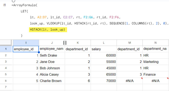
Formula_Expression
In the previous step, we combined two tables, and it wasn’t an inner join. As you can see, not all records in the left table have matches in the right table.
You need to filter out those rows because an inner join specifically means including only the matching records from both tables. The following FILTER function accomplishes this.
FILTER(merge, CHOOSECOLS(look_up, 1)<>"")(formula_expression): This filters themergearray based on the first column of thelook_uparray.CHOOSECOLS(look_up, 1)extracts only the first column oflook_up, containing matching values or #N/A error values.<>""checks if the values in this extracted column are not empty strings or #N/A error values, which would indicate a successful match and non-zero / non-error values.
Ultimately, this filter removes rows from the merge array where no matching value was found in the right table for the corresponding ID.
Conclusion
Mastering the inner joining of two tables in Google Sheets enables precise data combination and analysis.
This tutorial guides you through seamless inner joins in Google Sheets, providing essential knowledge for a deeper understanding of data relationships.
Integrate the insights from this tutorial into your workflow to elevate your Google Sheets expertise and streamline data analysis. Explore additional tutorials and review our sample sheet with formulas for further guidance.
- How to Left Join Two Tables in Google Sheets
- How to Right Join Two Tables in Google Sheets
- How to Full Join Two Tables in Google Sheets
Happy data crunching!


