In Google Sheets, a right join merges data from two tables, keeping all records from the right table and including matching records from the left table.
This join guarantees preserving all data from the right table, even if certain values lack corresponding entries in the left table.
The right table should have unique values in the common field for an effective right join. This precaution helps prevent ambiguity and ensures accurate data merging.
Note: If you have duplicated IDs in both ID columns (left and right tables), please check out this guide: Conquer Duplicate IDs: Master Left, Right, Inner, & Full Joins in Google Sheets.
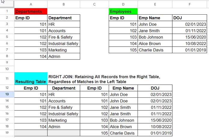
Right Join Two Tables: Sample Tables and Resulting Table
This example illustrates a right join scenario where the left table contains departments, and the right table contains employee names and their date of joining.
Table 1: Departments
| Emp ID | Department |
| 101 | HR |
| 101 | Accounts |
| 102 | Fire & Safety |
| 102 | Industrial Safety |
| 103 | Marketing |
| 104 | Admin |
Table 2: Employees
| Emp ID | Emp Name | DOJ |
| 101 | John Doe | 02/01/2023 |
| 102 | Jane Smith | 01/11/2022 |
| 103 | Bob Johnson | 15/06/2020 |
| 104 | Alice Brown | 10/08/2022 |
| 105 | Charlie Davis | 01/01/2019 |
Employee ID serves as the common field in both tables, enabling a right join. Importantly, the right table has unique records for employee IDs.
The result would be a combined table containing all employee records from the right table, along with their corresponding department information (if available) from the left table.
Expected Result:
| Emp ID | Department | Emp ID | Emp Name | DOJ |
| 101 | HR | 101 | John Doe | 02/01/2023 |
| 101 | Accounts | 101 | John Doe | 02/01/2023 |
| 102 | Fire & Safety | 102 | Jane Smith | 01/11/2022 |
| 102 | Industrial Safety | 102 | Jane Smith | 01/11/2022 |
| 103 | Marketing | 103 | Bob Johnson | 15/06/2020 |
| 104 | Admin | 104 | Alice Brown | 10/08/2022 |
| 105 | Charlie Davis | 01/01/2019 |
Please scroll down to see the screenshot of the above tables in Google Sheets.
Array Formula for Right Joining Two Tables in Google Sheets
To execute a right join on two tables in Google Sheets, a complex formula involving several functions can be utilized. However, you only need to specify the table ranges and unique identifier column ranges, and the formula will handle the rest.
Here’s the formula for performing a right join on two tables, assuming the right table has unique records in Google Sheets.
Formula:
=ArrayFormula(
     LET(
          lt, A2:B8, lt_id, A2:A8, rt, D2:F7, rt_id, D2:D7,
          merge1, REDUCE("", rt_id, LAMBDA(a, v, IFNA(VSTACK(a, HSTACK(v, FILTER(lt, lt_id=v)))))),
          key, SCAN("", CHOOSECOLS(merge1, 1), LAMBDA(a, v, IF(v="", a, v))),
          merge2, HSTACK(merge1, VLOOKUP(key, HSTACK(rt_id, rt), SEQUENCE(1, COLUMNS(rt), 2), 0)),
          CHOOSEROWS(CHOOSECOLS(merge2, SEQUENCE(1, COLUMNS(merge2)-1, 2)), SEQUENCE(ROWS(key)-1, 1, 2))
     )
)
After right joining two tables, you may need to apply ‘Format > Number > Date’ to any column that contains date values. You can find the right join array formula in cell A12 of the third sheet in the provided sample sheet below.
Anatomy of the Right Join Formula
The right join formula utilizes the LET function to assign ‘name’ to ‘value_expression’ results and returns the result of the ‘formula_expression’, which represents the resulting table from the right join.
Syntax of the LET Function:
LET(name1, value_expression1, [name2, …], [value_expression2, …], formula_expression)LET Assignments
lt(name1): Defines the data range of the left table, including the header row.A2:B8(value_expression1): Data range of the left table.
lt_id(name2): Defines the ID column of the left table, including the header row.A2:A8(value_expression2): ID column of the left table.
rt(name3): Defines the data range of the right table, including the header row.D2:F7(value_expression3): Data range of the right table.
rt_id(name4): Defines the ID column of the right table, including the header row.D2:D7(value_expression4): ID column of the right table.
Note: When employing the formula above for a right join of two tables in Google Sheets, you only need to adjust the value_expressions 1 to 4 according to your specific table configurations.
Other LET Assignments
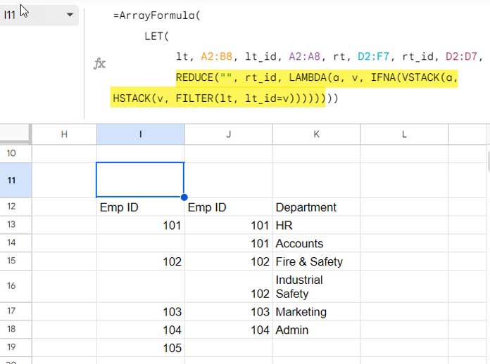
REDUCE Part:
merge1(name5)REDUCE("", rt_id, LAMBDA(a, v, IFNA(VSTACK(a, HSTACK(v, FILTER(lt, lt_id=v))))))(value_expression5): Filter the rows in the left table that match the Emp ID in the right table, and horizontally stack the Emp ID column from the right table with the corresponding rows from the left table (please refer to the image below).FILTER(lt, lt_id=v): This FILTER function extracts rows from the left table (lt) where the left table’s Emp ID (lt_id) matches the current element (v) from the right table’s Emp ID (rt_id).HSTACK(v, FILTER(lt, lt_id=v)): This function stacks the current element (v) horizontally with the result of the FILTER function (potentially multiple records from the left table). Empty cells may appear if the filter returns more than one record.- REDUCE with LAMBDA: This function iterates through the right table’s Emp ID (
rt_id) array and applies the provided LAMBDA function to each element. The LAMBDA function vertically stacks the accumulated result of HSTACK (current element + matching left table records) in each iteration.
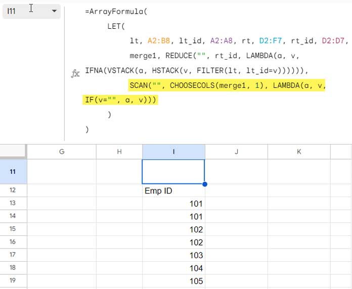
SCAN Part:
key(name6)SCAN("", CHOOSECOLS(merge1, 1), LAMBDA(a, v, IF(v="", a, v)))(value_expression6): Fill blank cells in the first column ofmerge1(REDUCE part) with the values from the cell above.- The SCAN function starts with an empty accumulator (
""). - It iterates through each cell in the first column (
CHOOSECOLS(merge1, 1)). - The LAMBDA function checks the current element (
v). - If
vis an empty string, it uses the accumulator value (a) and updates the accumulator. - If
vis not an empty string, it uses the current element value (v) and updates the accumulator.
- The SCAN function starts with an empty accumulator (
This achieves the intended behavior of filling in gaps in the first column of the merge1 table.
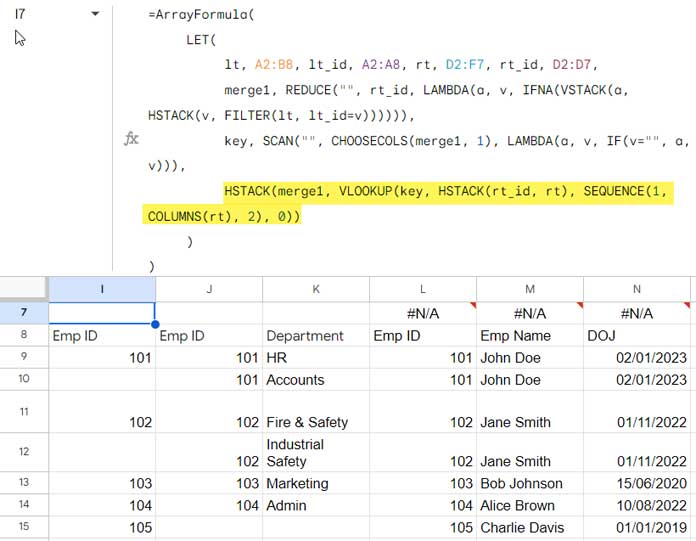
HSTACK and VLOOKUP Part:
This section performs a right join between two tables. However, the result may include an undesired row and column.
merge2(name7)HSTACK(merge1, VLOOKUP(key, HSTACK(rt_id, rt), SEQUENCE(1, COLUMNS(rt), 2), 0))(value_expression7): This formula combines themerge1(Reduce part) table with the results of a VLOOKUP lookup based on thekey(SCAN part) value. Let’s break it down step-by-step:
- HSTACK(merge1, …):
- HSTACK horizontally stacks two or more tables or ranges.
- Here, it combines the existing
merge1table with the results of the VLOOKUP lookup.
- VLOOKUP(…):
- This section executes a
VLOOKUPto matchkeyvalues in the right table (rt) and retrieve corresponding values. It will match all the key values since these keys are derived in a prior step from the right table itself. The only distinction is that the key may include multiple occurrences of Emp IDs, depending on how often they appear in the left table. VLOOKUP(key, …): searches for thekeyvalue within the specified range.HSTACK(rt_id, rt): Defines the range for the search. It merges thert_idcolumn with the entirerttable. This meets the criteria for VLOOKUP as it searches the first column of the lookup table for the search keys.SEQUENCE(1, COLUMNS(rt), 2): specifies which columns to return from therttable. It starts at column 2 (excluding thert_idcolumn) and returns all subsequent columns.
LET Formula Expression
CHOOSEROWS(CHOOSECOLS(merge2, SEQUENCE(1, COLUMNS(merge2)-1, 2)), SEQUENCE(ROWS(key)-1, 1, 2))We aim to exclude the first row (a row with blank or N/A values) and the first column (containing the rt_id column with blanks) from the result. To achieve this, we utilize CHOOSEROWS and CHOOSECOLS.
- CHOOSECOLS(merge2, SEQUENCE(1, COLUMNS(merge2)-1, 2)):
CHOOSECOLSselects specific columns from a table or range.merge2is the combined table created in the earlier part of the formula.SEQUENCE(1, COLUMNS(merge2)-1, 2)Defines the columns to be selected. It generates a sequence that matches the number of columns inmerge2minus 1, starting from 2. This effectively chooses all columns except the first one.
- CHOOSEROWS(…):
CHOOSEROWSselects specific rows from a table or range based on row index criteria.CHOOSECOLS(…)is the table containing the columns we want to select rows from.SEQUENCE(ROWS(key)-1, 1, 2)Defines the row indices to be selected. It generates a sequence starting from 2 up to one less than the total number of rows in thekeytable. This selects all the rows except the first row containing blanks or N/A.
Related Resources:


