The CHOOSEROWS function in Google Sheets generates a new array by selecting the specified row numbers from the existing range.

You can input positive or negative row number(s).

When negative row numbers are provided, the counting starts from the last row in the range (bottom to top), whereas it begins from the top when positive row numbers are used.

This function introduces various possibilities for data manipulation in Google Sheets.

For instance, the CHOOSEROWS function can be employed in conjunction with XMATCH and TOCOL to address a limitation of the XLOOKUP function.

What’s the limitation?

In situations involving multiple search keys, XLOOKUP will retrieve a value from a single column, even if the result_range contains more than one column.

We will delve into this in more detail below.

CHOOSEROWS Function — Syntax and Arguments

Syntax:

CHOOSEROWS(array, row_num1, [row_num2, …])

Arguments in the CHOOSEROWS Google Sheets Function:

• array: The source array or range.
• row_num1: The row number (in the array) of the first row to be returned.
• row_num2, …: The row number(s), if any, of additional rows(s) to be returned.

Row numbers can be positive or negative integers. If the row number isn’t an integer, the function will round it down.

Basic Usage

Suppose we have a table containing names, marks, and ranks of students, sorted based on rank, where the top rank holders appear first.

To retrieve the details of the 5th rank holder, excluding the header row, we can utilize the CHOOSEROWS function in Google Sheets.

=CHOOSEROWS(B3:D12, 5)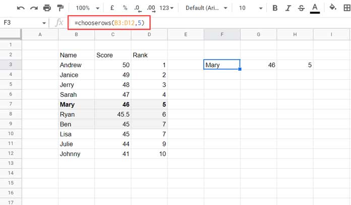

This function was introduced in 2023, and we had alternative solutions in the past. Here are those formulas:

1. Index.

=INDEX(B3:D12, 5, 0)

2. Query.

=QUERY(B3:D12, "SELECT * LIMIT 1 OFFSET 4", 0)

3. Offset.

=OFFSET(B3, 4, 0, 1, 3)

Now, let’s assume we want the details of the 5th, 6th, and 7th rank holders. To achieve this with the above formulas, we can use an array constant like {5, 6, 7} or SEQUENCE(3, 1, 5) within the CHOOSEROWS function in Google Sheets.

Examples:

=CHOOSEROWS(B3:D12, {5, 6, 7})
=CHOOSEROWS(B3:D12, SEQUENCE(3, 1, 5))

However, the INDEX function is not suitable for this purpose. Nevertheless, QUERY and OFFSET can handle this requirement effectively.

=QUERY(B3:D12, "SELECT * LIMIT 3 OFFSET 4", 0)
=OFFSET(B3, 4, 0, 3, 3)

CHOOSEROWS Function for Flipping a Table in Google Sheets

In my last tutorial, we explored how to flip a table from right to left using the CHOOSECOLS function in Google Sheets.

Similarly, we can achieve the same result of flipping a table, but this time from bottom to top, using the CHOOSEROWS function. Here’s how you can do it:

Assuming A2:D7 is the range to flip from bottom to top, you can use the following formula:

=CHOOSEROWS(A2:D7, SEQUENCE(ROWS(A2:A7), 1, -1, -1))

The SEQUENCE(ROWS(A2:A7), 1, -1, -1) generates a series of negative numbers from -1 to -7. As a result, the formula returns the rows from bottom to top.

Alternative Formula:

=SORT(A2:D7, SEQUENCE(ROWS(A2:A7)), 0)

This alternative formula achieves the same flipping effect by using the SORT function in conjunction with the SEQUENCE to sort the rows in descending order.

You may also be interested in: How to Flip a Column in Google Sheets – Finite and Infinite Columns.

XLOOKUP 2D Array Shortfall and Alternative Formula

Searching for required information manually in a large dataset can be time-consuming. Spreadsheet applications provide built-in lookup functions to streamline this process, and XLOOKUP is one of the popular choices.

With XLOOKUP, we can search for a key in a specified column of a table and retrieve the necessary information from all or specific columns. However, when attempting to search for multiple keys, XLOOKUP falls short as it only returns information from a single column.

Currently, the XLOOKUP function does not support returning a 2D array result. To overcome this limitation, we can utilize a combination of XMATCH, TOCOL, and CHOOSEROWS.

Here is an example illustrating this alternative approach.

CHOOSEROWS Function in Solving XLOOKUP Two-Dimensional Array Issue in Google Sheets

Problem:

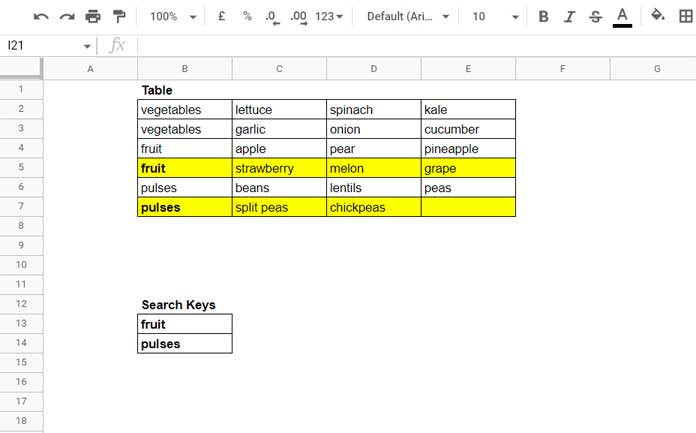
Search for “fruits” and “pulses” in the first column of the table and return the result from the entire row (except the first column), searching from the last entry to the first.

=ArrayFormula(XLOOKUP(B13:B14, B2:B7, C2:E7, "", 0, -1))

This formula will ONLY return “strawberry” and “split peas” from the first column of the result_range.

In this formula:

• search_key: B13:B14 (Two Search Keys)
• lookup_range: B2:B7 (The Range to Lookup)
• result_range: C2:E7 (2D Array)
• missing_value: “” (The Value to Return When There Is No Match)
• match_mode: 0 (Exact Match of the Search Keys)
• search_mode: -1 (Search from the Last Entry to the First)

Solution:

Let’s use the CHOOSEROWS function with TOCOL and XMATCH to solve the above problem.

=ArrayFormula(CHOOSEROWS(B2:E7, TOCOL(XMATCH(B13:B14, B2:B7, 0, -1), 3)))

Here is the XMATCH syntax:

XMATCH(search_key, lookup_range, [match_mode], [search_mode])

The XMATCH returns the row numbers for matching search keys and #N/A for mismatching ones.

The role of the TOCOL here is to remove the #N/A errors. Of course, we can use the IFNA for that. Still, it leaves a blank cell that may cause CHOOSEROWS to fail.

We have used those matching index numbers within the CHOOSEROWS function to return the relevant rows.