The CHOOSECOLS function in Google Sheets allows users to easily select specific columns from a range. It is often combined with the SEQUENCE function.
Introduced in 2023, this function provides a straightforward way to manipulate data without the complexity of older methods, which we will cover in a later section of this guide.
Syntax and Arguments
Syntax:
CHOOSECOLS(array, col_num1, [col_num2, …])Arguments:
- array: The source array or range from which you want to extract columns. This can be a direct range like A1:C10 or an array generated by other functions.
- col_num1: The column number (in the specified array) of the first column you want to return.
- col_num2,…: Additional column numbers to return (optional). You can specify multiple column numbers here.
Both positive and negative integers are accepted as column numbers. Positive integers count from the left, while negative integers count from the right.
If a value is not an integer, the function will round it down to the nearest whole number.
Using the CHOOSECOLS Function
Let’s take a look at some basic examples of how to utilize the CHOOSECOLS function effectively:
To return columns 2 and 4 from the left side of a specified array (for example, the range B2:E7):
=CHOOSECOLS(B2:E7, 2, 4)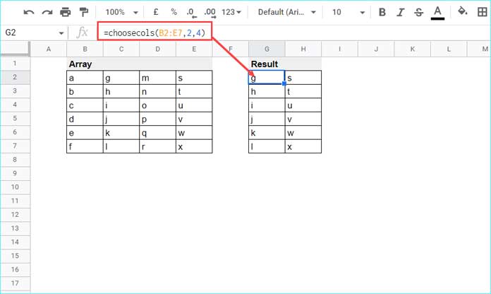
This formula extracts the second and fourth columns, allowing for targeted data analysis.
To retrieve the same columns but counting from the right side:
=CHOOSECOLS(B2:E7, -2, -4)This flexibility allows you to access columns regardless of their position in the original array.
The output will include the columns corresponding to the specified indices, which may contain specific values like letters or numerical data, depending on your dataset.
Selecting Multiple Columns
In the previous examples, we directly specified the column numbers. However, you can also use an array constant to select multiple columns more succinctly. For example, using {2, 4} as an argument for col_num1 allows for more dynamic selections:
=CHOOSECOLS(B2:E7, {2, 4})You can also integrate the SEQUENCE function to create a more complex selection.
Suppose you have monthly statuses across columns, with a blank column between each monthly column. You can use the SEQUENCE function to select only the relevant value columns:
=CHOOSECOLS(A1:G7, SEQUENCE(4, 1, 1, 2))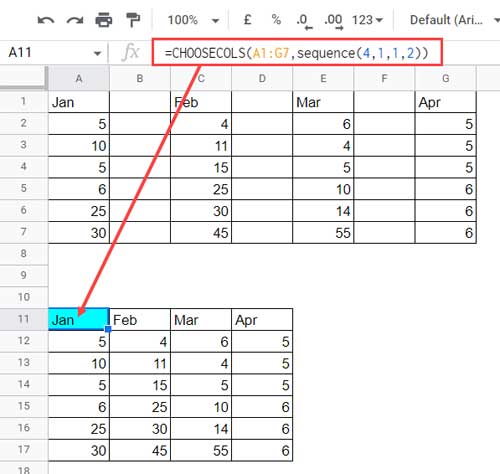
In this formula, SEQUENCE generates a list of four numbers in a single column, starting from 1, with a step of 2. As a result, the returned numbers will be 1, 3, 5, and 7, corresponding to the value columns you wish to extract.
Flipping a Table with CHOOSECOLS
The CHOOSECOLS function is not just for selecting; it can also be used to flip (reverse) a table horizontally. For instance, if you want to reorder columns from left to right (e.g., changing the order from Jan, Feb, Mar, Apr to Apr, Mar, Feb, Jan), you can achieve this with the following formula:
=CHOOSECOLS(A1:G7, SEQUENCE(4, 1, -1, -2))In this case, SEQUENCE generates the column indices starting from the end of the range and counting backward, allowing you to reverse the order effortlessly.
Popular Alternatives to CHOOSECOLS
While CHOOSECOLS is tailored for selecting columns, several alternative functions can also be used for similar purposes:
- INDEX: A versatile function that returns the value of a cell in a specific row and column within a given range.
=INDEX(A1:B, 0, 2)– This formula will return the second column from the specified range. - QUERY: A powerful function that allows you to run SQL-like queries on your data, making it easy to filter and manipulate datasets.
=QUERY(A1:B, "SELECT B")– This formula selects (returns) column B from the specified range. - OFFSET: This function returns a reference to a range that is a specified number of rows and columns from a given reference.
=OFFSET(A1, 0, 1, ROWS(A1:A))– This formula offsets 0 rows and 1 column, returning the second column because the height of the range is defined byROWS(A1:A).
Each of these functions has its strengths, but CHOOSECOLS stands out for its simplicity and direct focus on column selection.
Wrapping Up
The CHOOSECOLS function in Google Sheets is a game-changer when it comes to selecting specific columns from a range. Its introduction in 2023 brought a simpler, more intuitive alternative to some of the older methods like INDEX, QUERY, and OFFSET. By allowing you to pick columns easily and even reverse their order, CHOOSECOLS adds a new level of flexibility to your data manipulation.
Whether you’re using it to simplify column selection or combining it with functions like SEQUENCE for more dynamic results, CHOOSECOLS opens up new possibilities for efficiently organizing your data.
With the examples provided, you now have a solid understanding of how to leverage this function to streamline your work. So go ahead, apply the CHOOSECOLS function, and take your Google Sheets expertise to the next level!


