The QUERY function allows you to filter rows and select columns in a single step. This tutorial explains how to dynamically select every Nth column in QUERY, which is useful when filtering rows for specific items or categories and extracting alternate columns.
Why Select Every Nth Column?
You may need to extract alternate columns when working with structured data. For example, consider a table where employee names are in column A, and regular hours and overtime hours for each day are spread across subsequent columns. If you want to filter for a specific employee and extract only their overtime hours, you can use QUERY to select every alternate column dynamically.
Generic Formula:
=QUERY(data, "Select "&LET(cols, COLUMNS(data), seq, SEQUENCE(1, cols, startAt, Nth), JOIN(", ", ARRAYFORMULA("Col"&FILTER(seq, seq<=MAX(cols))))))Where:
- data – The data range to manipulate using the QUERY function.
- startAt – The starting column in the data range from which extraction begins.
- Nth – Determines the step value. If set to 2, it extracts every second column; 3 extracts every third column, and so on.
Additionally, if you want to include specific columns beyond the extracted Nth columns, specify them in the SELECT clause. By default, the formula starts with "Select ". If you want to include the first column, replace it with "Select Col1,". For the first and second columns, use "Select Col1, Col2,".
Example: Selecting Every Nth Column in QUERY
In the following example, we have employee names in column A and their regular and overtime hours in subsequent columns from Monday to Friday. The data range is A1:K in Sheet1.
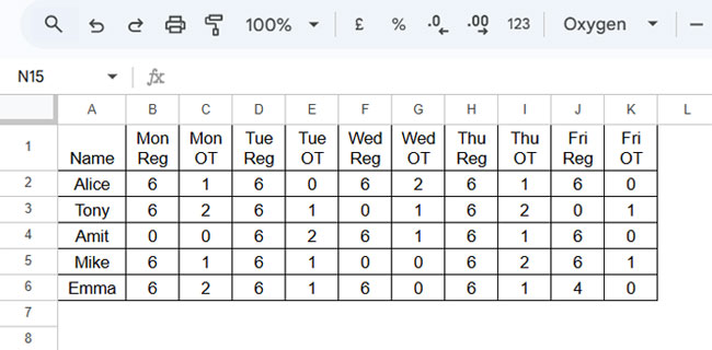
We want to select every second column from the third column onward, meaning all the overtime columns in the data range. Additionally, we want to include the first column (student names).
Here is the formula to select every Nth column in Google Sheets QUERY, adapted to this dataset and requirement:
=QUERY(Sheet1!A1:K, "Select Col1, "&LET(cols, COLUMNS(Sheet1!A1:K1), seq, SEQUENCE(1, cols, 3, 2), JOIN(", ", ARRAYFORMULA("Col"&FILTER(seq, seq<=MAX(cols))))))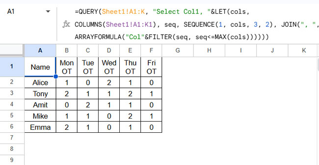
Explanation:
- data:
Sheet1!A1:K - startAt: 3 (third column, where overtime starts)
- Nth: 2 (every alternate column)
- Additional column: “Select Col1, ” (the column with student names)
This formula is equivalent to the following static QUERY formula:
=QUERY(Sheet1!A1:K, "Select Col1, Col3, Col5, Col7, Col9, Col11")We have automated the selection of columns by dynamically generating the part “Col3, Col5, Col7, Col9, Col11” and combining it with the rest of the QUERY statement.
For example, we dynamically create:
"Col3, Col5, Col7, Col9, Col11"and combine it with “Select Col1, “ as follows:
=QUERY(Sheet1!A1:K, "Select Col1, "&"Col3, Col5, Col7, Col9, Col11")To generate the column list dynamically, we use the following formula:
LET(cols, COLUMNS(Sheet1!A1:K), seq, SEQUENCE(1, cols, 3, 2), JOIN(", ", ARRAYFORMULA("Col"&FILTER(seq, seq<=cols))))This SEQUENCE formula generates a series of column numbers equal to the number of columns in the dataset. The starting value and step value determine which columns are selected. The “Col” text is concatenated with the column numbers. Additionally, FILTER ensures column numbers do not exceed the available columns, preventing errors.
How to Select Every Nth Column in QUERY and Filter Data
In the above example, we did not apply a row filter.
Assume we want to filter the rows where the student name is “Amit”. We need to add the following condition to the formula:
" where Col1='Amit'"Here’s the complete formula:
=QUERY(Sheet1!A1:K, "Select Col1, "&LET(cols, COLUMNS(Sheet1!A1:K1), seq, SEQUENCE(1, cols, 3, 2), JOIN(", ", ARRAYFORMULA("Col"&FILTER(seq, seq<=MAX(cols)))))&" where Col1='Amit'")Output:
| Name | Mon OT | Tue OT | Wed OT | Thu OT | Fri OT |
| Amit | 0 | 2 | 1 | 1 | 0 |
This method ensures that you filter both rows and select every Nth column dynamically in Google Sheets.
Conclusion
You can also use the CHOOSECOLS function combined with SEQUENCE to select every Nth column. However, CHOOSECOLS lacks the ability to filter rows. Another option is the FILTER function, but it cannot filter both rows and columns together unless nested with additional formulas.
Thus, QUERY is the best function to select every Nth column dynamically while also applying row filters.
Related Resources
- Dynamic Column References in Google Sheets Query
- How to Sum Every Nth Row or Column in Google Sheets
- How to Highlight Every Nth Row or Column in Google Sheets
- How to Copy Every Nth Cell from a Column in Google Sheets
- INDEX MATCH Every Nth Column in Google Sheets
- Delete Every Nth Row in Google Sheets Using Filters
- Import Every Nth Row in Google Sheets Using Query or Filter
- Date Sequence Every Nth Row in Excel


Why not simply
=JOIN(", ",ArrayFormula("Col"&SEQUENCE(COLUMNS(A1:Z)/3,1,COLUMN(A1)+3-1,3)))Hi,
Thanks for sharing.
This is exactly what I needed. I don’t pretend to know how or why it works, it just works.