If you want to highlight every nth row or column in Google Sheets, you can achieve this using the MOD function with Conditional Formatting. This technique is useful for visual clarity in your sheet and demonstrates how flexible functions like MOD can be. In this tutorial, you’ll learn how to highlight every nth row or column with step-by-step instructions and custom formulas.
How to Highlight Every Nth Row or Column in Google Sheets
To highlight rows, we use the ROW function with MOD. To highlight columns, replace ROW with COLUMN in the MOD formula. Here’s how to do it.
Highlight Every Nth Row in Google Sheets
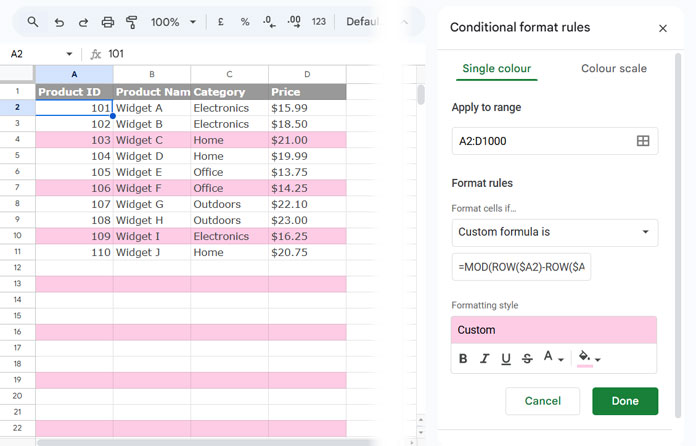
Assume you have sample data in the range A1:D, with the headers located in row 1. If you want to highlight every third row starting from the second row onward, leaving the header row intact, you can use the combination of the MOD and ROW functions. You can also adjust the divisor in the MOD function to highlight rows at different intervals.
Formula:
=MOD(ROW($A2)-ROW($A$2)+1, 3)=0Syntax: MOD(dividend, divisor)
Breakdown:
ROW($A2) - ROW($A$2) + 1: This part makes the first row in your range act like row 1. For example, if you’re starting from A2, it treats A2 as row 1 to highlight.MOD(…, 3) = 0: This function divides the relative row number by 3 and checks if the remainder is zero. This condition returns TRUE for every 3rd row, allowing the conditional formatting to be applied.
Applying Conditional Formatting
- Select the range where you want to apply the highlighting (e.g., A2:D, leaving the header row).
- Go to Format > Conditional Formatting.
- Enter the formula
=MOD(ROW($A2)-ROW($A$2)+1, 3)=0in the Custom Formula field. - Choose your desired formatting style and click Done.
This will highlight every 3rd row starting from the second row in your selected range.
Example for a Different Data Range
If your data range is different, for example, you want to highlight every nth row in the range C10:X100, the formula would be:
=MOD(ROW($C10)-ROW($C$10)+1, n)=0Replace n with the number of rows you wish to highlight at intervals.
Highlight Every Nth Column in Google Sheets
Just like row highlighting, you can highlight every nth column by using the COLUMN function instead of the ROW function.
In the previous examples, the cell reference in the first part was relative to the row, while the second part used an absolute reference. For column highlighting, the second part remains the same, but the first part should have a relative column reference.
To highlight every third column in the range A1:J, use the following formula in the Custom Formula field under conditional formatting:
=MOD(COLUMN(A$1)-COLUMN($A$1)+1, 3)=0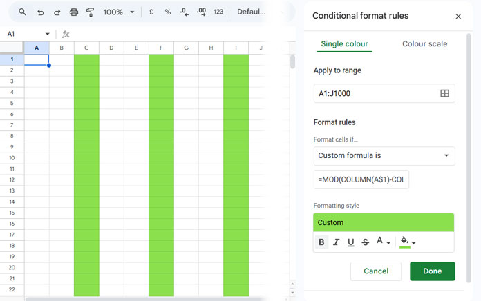
Example for a Different Data Range
If your data range is D10:Z100 and you want to highlight every fourth column, the formula would be:
Formula:
=MOD(COLUMN(D$10)-COLUMN($D$10)+1, 4)=0Final Tips:
- Format the Result Cells: After applying these formulas, format the result cells as desired.
- Adjust the Divisor: Modify the divisor in MOD to highlight every nth row or column at your preferred interval.
Conclusion
Using the MOD function with ROW or COLUMN in conditional formatting is a simple yet powerful way to highlight every nth row or column in Google Sheets. By adjusting the divisor, you can easily customize the pattern to suit different data layouts and improve readability.
For more practical conditional formatting techniques and advanced examples, explore the complete guide here: The Ultimate Guide to Conditional Formatting in Google Sheets


This was very helpful, thank you!
I don’t know what date the article was written, but nowadays (2019) the correct way to write the formulas is to use the semicolon
;to concatenate the formatting requests and not the comma,anymore.Hi, Fernando,
That depends on your region. I hope you are from one of the EU countries. Here we use the comma separator.
Related: How to Change a Non-Regional Google Sheets Formula.