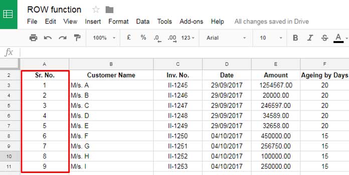
Auto Serial Numbering in Google Sheets with Row Function

Multiple Ways of Serial Numbering in Google Sheets:

As you may know, a standard format typically begins with a serial number column. To be more precise, this format may include columns such as serial number, description, client name, etc. The serial number column allows you to number rows in various ways. In this tutorial, we will explore auto-serial numbering in Google Sheets.

There are multiple ways one can adopt to insert serial numbers in Google Sheets. Before delving into dynamic methods for auto-numbering rows, it’s important to understand other available options that may be useful for beginners.

At the end of this post, I have also shared information on how to auto-increment alphabets as well as Roman Numerals in Google Sheets.

So, let us begin with different methods for auto serial numbering in Google Spreadsheet.

Standard format table with a serial number column in Google Sheets

Auto Serial Numbering Using Simple Formula

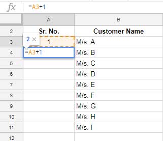
In the above example screenshot, our serial numbering starts from row #3, i.e., from cell A3.

First, enter 1 in cell A3. In cell A4, use the formula =A3+1 and then copy and paste this formula down to the cells below.

Serial numbers generated using a simple formula in Google Sheets

This method is commonly used for numbering in Google Sheets or Excel spreadsheets. It automatically adjusts row numbering when inserting or deleting rows in between.

Auto Row Numbering Using the Fill Handle

The fill handle behaves differently in Excel and Google Sheets.

For example, in Excel, you may enter 1 in cell A3 and 2 in cell A4. Then, select both cells and drag the fill handle down. This method may not work in Google Sheets.

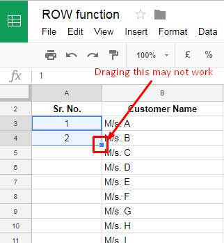
Serial numbering generated using the fill handle in Google Sheets

In Google Sheets, you do not need to select both cells. Just go to cell A4, then drag the fill handle down.

However, one thing is common in both. If you have values in the adjoining columns, left or right of the serial number column, double-clicking on the fill handle will fill the row numbers. In Excel, select both cells; in Google Sheets, only select the second cell.

Automatically Put Serial Number in Google Sheets Using the Row Function

Here, I’ve used the ROW function. This function can return the row number of a specified cell.

Syntax:

ROW([cell_reference])

Example:

=ROW(A3) // returns 3

The following formula will return the row number of the formula-applied cell.

=ROW()

Now, back to our topic:

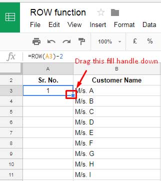
To get row numbering from row #3 (cell A3) downwards, enter the following formula in cell A3 and drag the fill handle down:

=ROW(A3)-2

The ROW function applied in cell A3 is =ROW(A3), which will return the row number 3 in the active cell. However, we need our serial number to start from 1. So, I have deducted 2 from it.

When you delete any row in between, in this case also, the serial number will automatically adjust.

If you want to start numbering from row #5, you should use =ROW(A5)-4. I hope it’s clear to you now.

Dynamic Auto Serial Numbering in Google Sheets

The ultimate way of auto serial numbering in Google Sheets!

The best option to automatically fill the serial numbers in Google Sheets is to use an array formula. You can either use the ROW function or the SEQUENCE function.

Row-Based:

If you want to get serial numbers 1 to 10 from cells A3 to A12, enter the following formula in cell A3:

=ArrayFormula(ROW(A3:A12)-2)

You only need to apply the formula in cell A3. No need to copy and paste it down. It will automatically number the cells below.

The ROW function with the support of the ArrayFormula returns the row numbers 3 to 12. We subtracted 2 from them to convert those outputs to 1 to 10.

Sequence-Based:

Another way to auto serial numbering is to use the SEQUENCE function. It’s an array formula. You just need to specify the number of sequences you want.

To get sequence numbers 1 to 10, use the following formula:

=SEQUENCE(10)

Conclusion

Although generating auto serial numbers using the SEQUENCE function is simple, the majority of Sheets’ users depend on the ROW function. This is because the SEQUENCE function is relatively new.

The purpose of the ROW function is to return the row numbers. However, we can also use it for auto-serial numbering. On the other hand, the SEQUENCE function is a dedicated function for returning sequence numbers with more features such as specifying the starting number of the sequence and step value. Additionally, it can return results in a 2D array.

Resources

17 COMMENTS

Bea Avaria December 9, 2021 At 3:46 pm

I just wanna leave a ‘thanks’ here because this article helped me so much to be more efficient, thank you for sharing!

InternQuesions May 23, 2021 At 12:55 am

Hi – I will try to explain it as best as I can. Do you know how I can do this in google sheets?

When I write something in B3, I want the number “1” to appear in A3. When I type something in B7, I want the number “2” to appears in A7. When I write something in B20, I want the number “3” to appear in A20, and so forth.

So essentially I want the number sequence to continue based on which row I type information into.

Is this possible?!

- Prashanth May 23, 2021 At 5:37 pm
  
  Hi, InternQuesions,
  
  That might be possible with Apps Script. But, sorry to say, I don’t have the solution to offer.
  
Adrienne December 16, 2020 At 1:04 am

Hello – I am trying to enter “Payroll 1” into cell A17; “Payroll 2” into cell A33 and so-on for multiple sheets within the same workbook (there are dates in rows/cells between). I’d like for the numbers after the word ‘Payroll’ to increment by 1, by referencing the previous ‘Payroll X’ cell. I cannot seem to figure out a formula to make this work, would you please be able to help?

- Prashanth December 16, 2020 At 4:38 pm
  
  Hi, Adrienne,
  
  I assume you have the string “Payroll 1” in cell A17. Then you want “Payroll 2” in cell A33 but between A17 and A33 there are values.
  
  In cell A17 manually enter the string “Payroll 1”. In cell A33, insert the below formula.
  
  ="Payroll "&countif($A$1:A32,"Payroll*")+1
  
  Then copy-paste this formula in any cells down to increment the number to “Payroll 3” and so on.
  
Trang May 14, 2020 At 8:59 pm

Hi Prashanth,

I want to fill in Week 1, Week 2, Week 3, up to Week 13, and then repeat four times.

That’s because each quarter has 13 weeks (based on a project management model), and four times represent four quarters of the year.

- Prashanth May 15, 2020 At 10:46 am
  
  Maybe this.
  
  =ArrayFormula("Week "&sequence(13,1))
  
  - Trang May 19, 2020 At 9:54 am
    
    Sorry I didn’t get back to you sooner. What if I want to repeat that Week 1-Week 13 several times, so that I have 52 rows, as in 52 weeks in a year?
    
    - Prashanth May 20, 2020 At 2:24 pm
      
      Hi, Trang,
      
      =ArrayFormula(transpose(split(textjoin("|",1,if(row(A1:A3), textjoin("|",1,"Week "&sequence(13,1))),),"|")))
      
      In this formula (13,1) for Week # 1 to 13.
      
      The formula part (A1:A3) is for repeating the week # 1 to 13, 3 times.
      
      - Trang May 21, 2020 At 8:18 am
        
        Thank you, Prashanth for taking the time to help me. What a monster formula. After half an hour, I finally understand it.
        
Stece January 16, 2020 At 9:39 pm

The downside of using the Row() Function is that if you add a Data filter and use sorting on that spreadsheet, your ID’s column will not work anymore. The numbers stay the same, even though the order of your records has changed.

Any solution for that?

- Prashanth January 17, 2020 At 9:55 am
  
  Hi, Stece,
  
  Yes! When using the auto serial numbers, the issue with filtering/sorting is there. Because the generated numbers have no direct relationship with the data in adjoining columns. If it was not the case, I mean if the array formula has some connection, then there is a workaround – how to Stop Array Formula Messing up in Sorting in Google Sheets.
  
  So, the workaround is to go for Query function to filter as well as sort the data in another tab.
  
  For example B1:B contains auto serial numbers generated using the ROW or SEQUENCE function and C1:C contains some product names (in ‘Sheet1’).
  
  To sort the product names in ‘Sheet2’, use the Query as below.
  
  =query(Sheet1!B1:C,"where C is not null order by C asc,1")
  
  To include filter, like sort the column C in Asc order and then filter the items “product 1”, “product 2” and “product 3”, use the below Query.
  
  =query(Sheet1!B1:C,"where C matches 'product 1|product 2|product 3' and C is not null order by C asc,1")
  
  Note: Filtering is case sensitive.
  
  To learn Query, open my Google Sheets Function Guide. To master Query filtering, read this guide – The Alternative to SQL IN Operator in Google Sheets Query (Also Not IN).
  
ravi September 10, 2019 At 3:54 pm

Super bro

Paulo May 6, 2019 At 5:32 am

I achieved the same with a more convoluted formula.

=IF(ISBLANK(B2);"";ARRAYFORMULA(ARRAY_CONSTRAIN(row(B2:B); COUNTA(FILTER(B2:B;LEN(TRIM(B2:B))>0));1)-1))

You made good use of the logic operators. I didn’t know it worked that way. Thanks!

- George October 31, 2019 At 5:53 pm
  
  Your convoluted formula worked, not the simple logical one offered in this article!
  
  - Prashanth November 1, 2019 At 12:49 pm
    
    Hi, George,
    
    If you are looking for a simple formula to populate serial numbers, then you can try this also.
    
    Empty a column and apply this formula in any cell in that column for serial numbers 1 to 100.
    
    =SEQUENCE(100,1)
    
    If you want the same in a row, empty a row, and use this one.
    
    =SEQUENCE(1,100)
    
    Best,
    
    - Levi November 26, 2019 At 11:28 am
      
      Thanks!!! This is what I’ve been looking for 😀