If you want to number a list in reverse order, such as from 50 to 1, you can use a formula to generate a backward sequence in Google Sheets.
In this tutorial, I will explain how to generate backward/reverse sequence numbers in Google Sheets using both a custom base value and a dynamic base value.
For example, if the base value is 10, the numbering (counting pattern) would be 10, 9, 8, and so on. Additionally, you will learn the following:
- Backward sequence numbering while leaving blank cells in the list (dynamic base value).
Backward Sequence Numbering Based on a Base Value
Assume the base value is 10. To get sequence numbers backward from 10 to 1, you can use the following formula:
=SEQUENCE(10, 1, 10, -1)This formula generates 10 numbers in 1 column, starting from the base value of 10. The step value of -1 ensures that the sequence decreases by 1, resulting in a backward sequence from 10 to 1.
Syntax:
SEQUENCE(rows, [columns], [start], [step])Here, you specify the base value (10) for the number of rows (rows) and the starting value (start).
When using this formula, replace both occurrences of 10 with your desired base value. No other changes to the formula are required.
Dynamic Backward Sequence Numbering in Google Sheets
In the earlier example, we used a static base value of 10. But what if you want to generate backward sequence numbers without a fixed base value, using a dynamic base instead?
This becomes especially useful when you want to number a list in descending order, which may grow or shrink over time.
For instance, if you have 30 names in column A (range A2:A31), the list may grow as you add more names. The backward sequence should automatically adjust, starting from the total number of rows (e.g., 30) and counting down as new rows are added.
To achieve this, replace the static base value in the earlier formula with a dynamic base value:
ArrayFormula(XMATCH(TRUE, A2:A<>"", 0, -1))This formula counts the number of non-blank rows from the start of the list to the end. Currently, it will return 30, and as the list grows, this number will update accordingly.
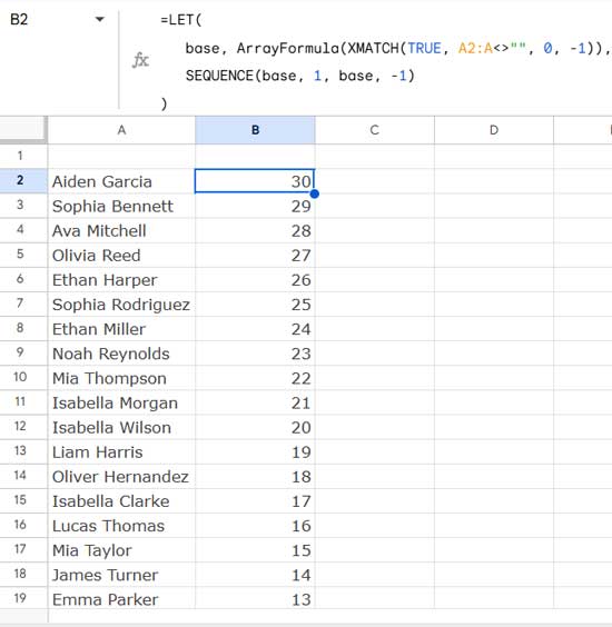
Now, the formula in cell B2 would be:
=SEQUENCE(ArrayFormula(XMATCH(TRUE, A2:A<>"", 0, -1)), 1, ArrayFormula(XMATCH(TRUE, A2:A<>"", 0, -1)), -1)In this case, the formula for both rows and start is the same. To optimize performance and readability, you can use the LET function:
=LET(
   base, ArrayFormula(XMATCH(TRUE, A2:A<>"", 0, -1)),
   SEQUENCE(base, 1, base, -1)
)
This is the dynamic formula for backward sequence numbering in Google Sheets.
When using this formula, replace A2:A with the range corresponding to the list for which you want to apply the reverse sequence.
Skipping Blank Rows in Backward Sequence Numbering
Sometimes, blank rows are left between data entries for formatting purposes or due to removed values, but you don’t want these rows to receive a backward sequence number. Here’s how to handle that.
If you replace the earlier formula in cell B2 with this updated one, you will get the same sequence from 30 to 1. The backward sequence will grow or shrink as the list grows or shrinks, and it will only place numbers in non-blank rows:
=ArrayFormula(IF(A2:A="",,COUNTIFS(A2:A,"<>", ROW(A2:A), ">="&ROW(A2:A))))The COUNTIFS function counts non-blank cells in the range A2:A, and ensures that only rows with values in column A receive a sequence number.
The last condition compares the row numbers, so the backward sequence will count from the last non-blank row upwards. The IF function ensures that numbers are only placed in non-blank rows.
Resources
- Fill a Column with Sequence of Decimals in Google Sheets
- Sequence Numbering in Merged Cells in Google Sheets
- Create a Dynamic Fibonacci Sequence in Google Sheets
- Auto Serial Numbering in Google Sheets with Row Function
- Group-Wise Serial Numbering in Google Sheets
- Skip Hidden Rows in Sequential Numbering in Google Sheets
- Assign Same Sequential Numbers to Duplicates in a List in Google Sheets


