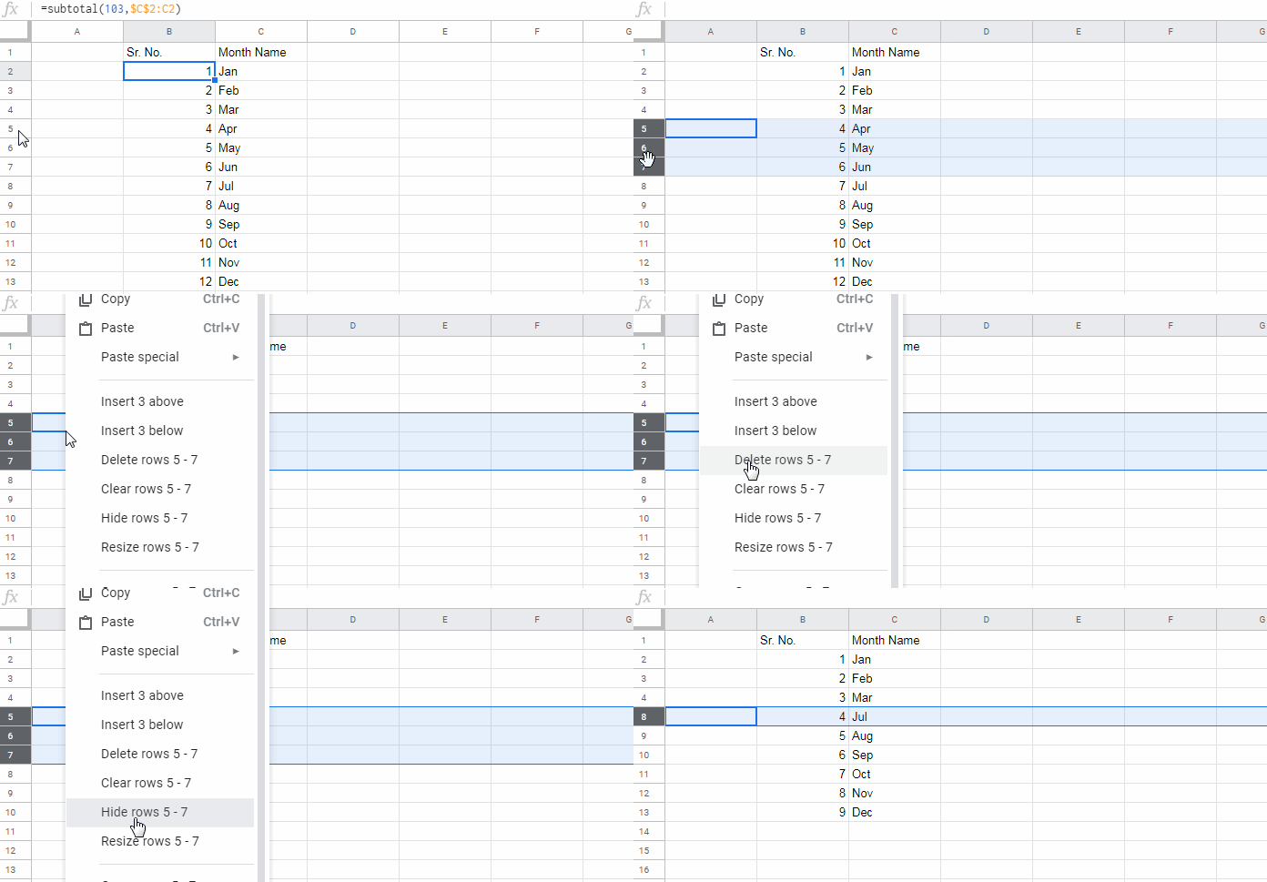
This post is about how to insert sequential numbers skipping hidden rows in Google Sheets. Hidden (invisible) rows are the rows that not visible due to grouping, filtering, right-click row hide, etc.
With the introduction of the SEQUENCE function, in Google Sheets, it’s pretty easy to generate sequential numbers, sequential dates, etc.
There is one more equally important function to generate sequential numbers and it’s as you may already know the ROW function.
In our case, none of the above functions (SEQUENCE or ROW) would work because of the lack of functionality in identifying hidden rows.
The only function capable of distinguishing a hidden (invisible) row from an unhidden (visible) row is the SUBTOTAL in Google Sheets.
Using the said function, let’s see how to fill down serial/sequential numbers skipping hidden rows in Google Sheets.
Below you will get the step by step instructions to do the same.
How to Insert Sequential Numbers Skipping Hidden Rows in Google Sheets
As I have mentioned, to insert sequential numbers skipping hidden rows we can use the SUBTOTAL function in Google Sheets. Here is an example.
I have the below list in column C and I want to insert sequential numbers in column B that only in the visible rows.
See how I am achieving that with a SUBTOTAL formula.

The list starts from cell C2. So I want to start the numbering from cell B2.
The following SUBTOTAL formula in cell B2 dragged down to copy-paste it in other cells down.
=subtotal(103,$C$2:C2)It counts the rows until each row skipping blank rows but only will work well if there are no blank cells on the list. That hints about a drawback, right?
Actually there are two drawbacks of the above SUBTOTAL formula that skips hidden rows in sequential numbering. Here are those two said drawbacks.
- There should not be blank cells in the range (list) in column B. If there are any blank cell, at least put white space in that cell by tapping the spacebar or type the hidden character single apostrophe
('). - This second point is not associated with the above formula. It’s a drawback associated with the function itself, i.e. the SUBTOTAL won’t expand results. So we need the formula in each row to work. That’s why we are dragging the B2 formula down.
Some of you may want to keep the blank cells as blank only, right? Then there is a workaround with a helper column. See that below.
Helper Column to Avoid SUBTOTAL Counting Issues Due to Blanks
Let me explain why the helper column is required.
We have used a SUBTOTAL equivalent to COUNTA function (refer to the function # 103 used within the formula).
Actually, my formula is for counting rows with values in C2:C range, i.e. skipping blanks. That cause issue with unhidden black rows.
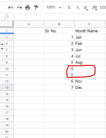
In the following example, the cells C10 and C11 are blanks and that makes issues in the sequential numbering using SUBTOTAL in Google Sheets.

To avoid such errors, I’ve suggested inserting an apostrophe character or white space here in cell C10 and C11. If you want to keep those cells blank, then follow this workaround.
Steps
Enter the below formula in cell E1.
=sequence(ArrayFormula(max(iferror(row(C2:C)/(C2:C<>"")))),1)It will generate sequential numbers up to the last row that contains the value in column C. Then hide column E (column E is now a helper column).
Now in cell B2 insert the following SUBTOTAL formula and then drag-down.
=subtotal(103,$E$2:E2)This will solve the issue.
That’s all about how to insert sequential/serial numbers skipping hidden rows in Google Sheets. Thanks for the stay. Enjoy!
Related Formula Examples
- Google Sheets Query Hidden Row Handling with Virtual Helper Column.
- SUMIF Excluding Hidden Rows in Google Sheets [Without Helper Column].
- How to Omit Hidden or Filtered out Values in Sum [Google Doc Spreadsheet].
- Vlookup Skips Hidden Rows in Google Sheets – Formula Example.
- Check Whether a Row Is Hidden and Highlight the Row above It.
- Find the Average of Visible Rows in Google Sheets.
- Count Unique Values in Visible Rows in Google Sheets.
- Highlight Visible Duplicates in Google Sheets.
- IMPORTRANGE to Import Visible Rows in Google Sheets.


