Highlighting Visible Duplicates in Google Sheets

Before we dive into highlighting visible duplicates in Google Sheets, let’s first understand what “visible duplicates” mean.

When a value appears more than once in a dataset, it is considered a duplicate. However, when dealing with visible duplicates, values in hidden rows are ignored. This means they are not counted when determining duplicate occurrences.

For example, if “blueberry” appears in cell A1 and A5, but A1 is hidden, then A5 is not considered a duplicate because it appears only once in the visible rows.

Customizing How Duplicates Are Highlighted

When applying a conditional formatting rule, you have three main options for highlighting visible duplicates in Google Sheets:

Highlight all occurrences of visible duplicates.
Highlight visible duplicates, except the first occurrence.
Highlight visible duplicates, except the last occurrence.

The last two options are useful when you want to remove duplicate rows by filtering based on fill color.

Highlighting All Occurrences of Visible Duplicates

Let’s consider a sample dataset in B2:B15, containing various fruit names. The data is sorted for easy understanding, but sorting is not required for the formula to work.

Use the following formula to highlight all occurrences of visible duplicates in the range B2:B15:

=LET(hr, MAP($B$2:$B$15, LAMBDA(row, SUBTOTAL(103, row))), COUNTIFS($B$2:$B$15, $B2, hr, CHOOSEROWS(hr, ROW($B2)-ROW($B2)+1))>1)

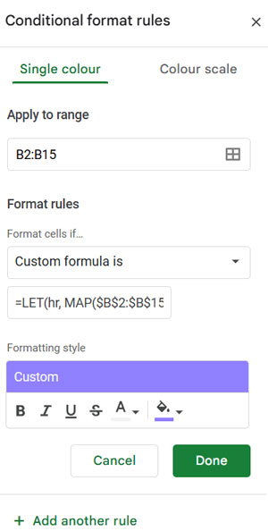
Google Sheets highlighting all visible duplicate values in a dataset

How to Apply the Rule:

Select B2:B15.
Click Format > Conditional Formatting.
Under Format rules, select Custom formula is.
Copy and paste the above formula.
Choose a highlighting style of your preference.
Click Done.

Google Sheets conditional formatting settings for applying a custom formula to highlight duplicates

This formula will highlight all visible duplicates in the selected range.

Formula Explanation

MAP($B$2:$B$15, LAMBDA(row, SUBTOTAL(103, row)))
- This is a helper formula named hr (hidden rows) that detects hidden rows. It returns 0 for hidden rows and 1 for visible rows.
COUNTIFS($B$2:$B$15, $B2, hr, CHOOSEROWS(hr, ROW($B2)-ROW($B2)+1))
- This counts the occurrences of each value only in visible rows.
- The condition ensures only visible duplicates are counted.

The formula highlights cells where the count is greater than 1, meaning duplicates are found in visible rows.

Highlighting Visible Duplicates Except the First Occurrence

Highlight Rule:

=LET(hr, MAP($B$2:$B2, LAMBDA(row, SUBTOTAL(103, row))), COUNTIFS($B$2:$B2, $B2, hr, CHOOSEROWS(hr, ROW($B2)-ROW($B2)+1))>1)

Use this formula instead of the previous one when you want to highlight visible duplicates while skipping the first occurrence of each value.

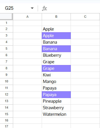
Google Sheets highlighting visible duplicates while leaving the first occurrence unhighlighted

How does this work?

Unlike the previous formula, this one counts occurrences only up to the current row, instead of the entire range.
The first occurrence will always have a count of 1, so it won’t be highlighted.

Highlighting Visible Duplicates Except the Last Occurrence

Highlight Rule:

=LET(hr, MAP($B2:$B$15, LAMBDA(row, SUBTOTAL(103, row))), COUNTIFS($B2:$B$15, $B2, hr, CHOOSEROWS(hr, 1))>1)

This formula highlights all visible duplicates except the last occurrence.

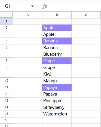
Google Sheets highlighting visible duplicates while leaving the last occurrence unhighlighted

How does this work?

The formula counts the occurrence of each value from the current row to the last row.
For example, if a value appears 3 times in visible rows, the counts will be 3, 2, 1.
Since the last row will have a count of 1, it won’t be highlighted.

Conclusion

We explored three advanced conditional formatting rules for highlighting visible duplicates in Google Sheets. These rules work without using a helper column.

However, keep in mind:

Highlighting large datasets may slow down performance, especially with complex formulas.
The formulas use the LAMBDA function, which may contribute to performance lag in Google Sheets.

By applying these methods, you can efficiently manage duplicate data while considering only visible rows.

3 COMMENTS

Grad Art July 8, 2019 At 10:50 pm

D’oh, that’s a bummer! Thanks for trying though.

Grad Art July 6, 2019 At 2:20 am

Hi, this is super, thanks Prashanth, got it to work great for a vertical range, i.e. same scenario as above. However, I’m also trying to get it to work on a separate sheet for a horizontal range, but can’t get it to work…I’ve tested & confirmed that the subtotal formula is not working for a horizontal instead of vertical scenario.

For example, my list is going across a single row, with the subtotal formulas set up on the row below that, but when I hide one of the columns, the subtotal formula in the hidden column still calculates to 1, instead of 0. Any ideas on how to make it work? Is there a different formula than subtotal that works for horizontal ranges instead of just vertical?

Thank you!

- Prashanth July 7, 2019 At 9:09 am
  
  Hi, Grad Art,
  
  For horizontal range, as you have tested, we can’t follow this method. I thought we can use the CELL function to find the width as below and use that in conditional formatting.
  
  =cell("width",E1)
  
  My assumption was it would return ‘0’ as the output when the Column E is hidden. But the column width remains the same. So I don’t have any option/workaround to offer.
  
  Best,