Conditional formatting based on data groups means highlighting each alternating category row or rows in a column in Google Sheets.

For example, if you have the category “apple” in A1:A5, “mango” in A6:A10, and “orange” in A11:A15, A1:A6 and A11:A15 will be highlighted with one color, while A6:A10 will either be left without highlighting or use another color.

In the following example, we have a category column A. Let’s explore how to apply alternating colors to groups of data in this column, with or without using a helper column.

Conditional Formatting Based on Data Groups Using a Helper Column

There are two key steps involved: preparing the helper column and applying the rule.

Step 1: Preparing the Helper Column:

We have data in column A where A1 contains the field label. Let’s choose column C as our helper column.

In cell C2, below the header row, enter the following formula:

=IF(A2=A1, N(C1), N(C1)+1)

Drag the fill handle of cell C2 down to the last cell where you want the formatting to apply (e.g., C12).

This copies the formula from C2 to C12 and segregates data into groups, assigning numbers like 1 for the first group, 2 for the second group, and so on.

The IF logical formula returns the value in the cell above in column C if A2 equals A1, or it returns the value in the cell above plus 1. The N function is used to handle non-numeric values, returning 0 for non-numbers and the value itself if it’s a number.

Step 2: Applying the Highlight Rules:

Now, let’s set up the highlight rule for conditional formatting based on data groups:

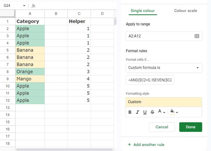
1. Select cells A2:A12 or up to the last row where you want to apply the alternating group colors.
2. Click on the Format menu > Conditional formatting.
3. Under Format rules, select “Custom formula is”.
4. Enter =ISODD($C2) in the formula field.
5. Choose your preferred formatting style under “Formatting style”.
6. Click “+ Add another rule”.
7. Enter =AND($C2>0, ISEVEN($C2)) in the formula field for the second rule.
8. Choose a different formatting style.
9. Click “Done”.

The highlight rules highlight even numbers in the helper column with one color and odd numbers with another color.

This completes the helper column approach for conditional formatting based on groups in Google Sheets.

Conditional Formatting Based on Data Groups Without Helper Column

Highlighting groups of data with alternating colors is much easier with the following XMATCH and UNIQUE combo.

Here, you don’t need the helper column C.

Follow all other steps from the previous approach but adjust the formulas:

In place of the ISODD formula, use =ISODD(XMATCH($A2, UNIQUE($A$2:$A))).

And for the ISEVEN formula, use =ISEVEN(XMATCH($A2, UNIQUE($A$2:$A))).

The UNIQUE function returns unique categories, while XMATCH matches each value and returns its relative positions.

For example, if the unique values are:

Apple
Banana
Orange
Mango

Then the relative positions are 1 for Apple, 2 for Banana, 3 for Orange, and 4 for Mango. XMATCH assigns these numbers based on matches in column A.

Resources

• Alternating Colors for Groups and Filtering Issues in Google Sheets
• Google Sheets – Highlight the Max Value in Each Group
• How to Highlight the Min Value in Each Group in Google Sheets
• Highlight Groups When Group Total Exceeds Target in Google Sheets
• Highlighting Multiple Groups and Control Tick Boxes in Google Sheets
• Applying Alternating Colors to Visible Rows in Google Sheets & Excel
• Google Sheets: Highlight Rows When Value Changes in Any Column
• Highlight the Latest Value Change Rows in Google Sheets
• Sum Column B When Value in Column A Changes in Google Sheets
• Customizing Alternating Colors of a Table in Google Sheets
• Find the Row Numbers of Change in Values in Google Sheets