When you have a dataset sorted by categories in Google Sheets, you might want to highlight rows when values change in the category column. This means highlighting either the first or the last row of each category.

This is useful when specific information, such as a subtotal, is found in the last or first row of each category.

To highlight the first row, you’ll need one formula, and for the last row, another formula.

The conditional formatting settings are the same, except for the formula. Let’s dive into the formulas and how to apply the highlight rules.

Quick Answer: Highlight Rows When Value Changes

Use these formulas in conditional formatting:

Highlight last row:

=$B2<>$B3

Highlight first row:

=AND($B2<>"", $B1<>$B2)

Example 1: Highlight the Last Row of Each Category

The sample data consists of student names in column A, divisions in column B, and their marks in column C. The data is sorted by division, and the last row of each division contains the division average.

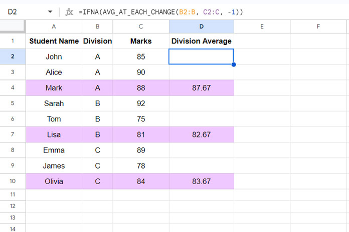
As a side note, I’ve used the following custom function in cell D2 to get the division average. You can import this function and similar aggregation functions from my guide: AT_EACH_CHANGE Named Functions in Google Sheets.

=IFNA(AVG_AT_EACH_CHANGE(B2:B, C2:C, -1))

Note: The custom function used here is optional. The highlighting formulas work independently without it.

To highlight the rows where the value changes in the division column, use the following conditional format rule:

=$B2<>$B3

Example 2: Highlight the First Row of Each Category

In this scenario, the average of each division is displayed in the first row of each division. The following custom function achieves that:

=IFNA(AVG_AT_EACH_CHANGE(B2:B, C2:C, 1))

To highlight the first row of each division, use the following conditional format rule:

=AND($B2<>"", $B1<>$B2)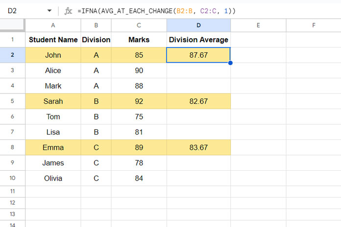

You might think that this highlighting can be achieved by simply matching non-empty cells in column D. However, my formula highlights the rows based on changes in column B, not just non-empty cells. I’m focusing on this approach because you may or may not have a subtotal column. The goal is to identify the rows where the group changes in your table. With that clarified, let’s move on to the steps for applying the above rules to highlight these rows.

How to Apply Conditional Formatting for Value Changes

You can choose one of the rules above based on your requirements. Copy that rule, then follow the steps below:

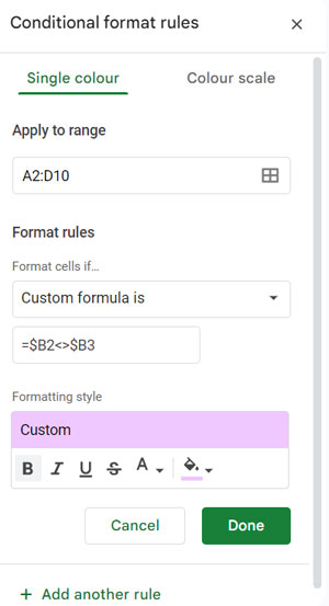
1. Select the range A2:D10 (or the range you want to highlight), avoiding the header row if there is one. In my case, A1:D1 contains the header, so I omitted that.
2. Click Format > Conditional Formatting.
3. In the sidebar panel, select “Custom formula is” under the “Format Rules.”
4. Paste the copied formula in the provided field. If your range is not A2:D10, modify the formula accordingly. For example, if your range is A10:Z100 and the category column is A, the formulas should be:
   • For the last row: =$A10<>$A11
   • For the first row: =AND($A10<>"", $A10<>$A9)
5. Select a highlighting style under “Formatting style.”
6. Click Done.

This way, you can highlight rows based on value changes in a column in Google Sheets.

Common Mistakes When Highlighting Value Changes

• Forgetting absolute references ($B2)
• Applying formula to wrong range
• Using incorrect row references
• Not sorting data before applying rules

Conclusion

Highlighting rows when values change in Google Sheets is a simple yet powerful way to visually separate grouped data. Whether you want to highlight the first or last row of each category, using custom conditional formatting formulas gives you full control without requiring helper columns.

These techniques are especially useful in reports, grouped datasets, and dashboards where identifying category boundaries is important.

This tutorial is part of The Ultimate Guide to Conditional Formatting in Google Sheets, which covers a wide range of techniques, examples, and advanced use cases for working with data more effectively.

Resources

• Find the Row Numbers of Change in Values in Google Sheets
• Filter Last Status Change Rows in Google Sheets
• Highlight the Latest Value Change Rows in Google Sheets
• Sum Column B Based on Changes in Column A in Google Sheets
• Automatically Insert Blank Rows Between Groups in Google Sheets
• Conditional Formatting Based on Data Groups in Google Sheets