The INDIRECT function is essential when you want to apply conditional formatting based on data from another sheet in Google Sheets.
In conditional formatting, you cannot directly reference a cell or range from a different sheet using a normal reference like:
='Student Group'!A1
To make cross-sheet references work, you must use the INDIRECT function.
This method is the foundation for applying conditional formatting based on data from another sheet in Google Sheets.
Quick Answer
You cannot directly reference another sheet in conditional formatting in Google Sheets. To do this, use the INDIRECT function to convert a text string into a valid reference.
For example:
=INDIRECT("Student Group!A1")
To highlight values based on another sheet:
=XMATCH(A2, INDIRECT("Student Group!B:B"))
Why INDIRECT Is Required in Conditional Formatting
Google Sheets restricts direct cross-sheet references inside conditional formatting rules.
The INDIRECT function solves this by converting a text string into a valid cell or range reference that conditional formatting can evaluate.
Syntax:
=INDIRECT("SheetName!Range")
Example: Highlight Names Based on Group from Another Sheet
Let’s consider two sheets:
- Student Group → Contains student names grouped under RED, BLUE, GREEN, and YELLOW
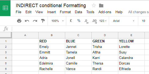
- Find Group → Contains a list of student names (e.g., winners)
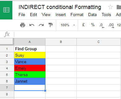
Goal: Highlight each name in the Find Group sheet based on the group they belong to in the Student Group sheet.
We will apply conditional formatting to range A2:A in the Find Group sheet.
Custom Formulas
Use the following formulas for each group:
=XMATCH(A2, INDIRECT("Student Group!B:B")) // Red
=XMATCH(A2, INDIRECT("Student Group!C:C")) // Blue
=XMATCH(A2, INDIRECT("Student Group!D:D")) // Green
=XMATCH(A2, INDIRECT("Student Group!E:E")) // Yellow
Each formula checks whether the name in A2 exists in the respective column of the Student Group sheet.
- If a match is found → returns a number → formatting is applied
- If not → returns #N/A → no formatting
How to Apply These Rules
- Go to the Find Group sheet
- Select the range A2:A
- Click Format > Conditional formatting
- Under Format cells if, choose Custom formula is
- Enter the first formula and set the color (e.g., Red)
- Click Add another rule and repeat for the remaining formulas
- Assign corresponding colors for each group
Now, when you enter a student name, it will automatically be highlighted based on the group.
Try this example yourself and see how the conditional formatting works across sheets.
Highlight Values Based on Another Sheet (Simple Example)
If you want to highlight values in column A based on whether they exist in another sheet, use:
=XMATCH(A2, INDIRECT("Sheet2!A:A"))
This checks whether the value in A2 exists in column A of another sheet.
Highlight Duplicates Across Sheets
To highlight duplicates between two sheets:
=COUNTIF(INDIRECT("Sheet2!A:A"), A2)
This highlights values in the current sheet that also appear in another sheet.
Common Issues with INDIRECT in Conditional Formatting
- Full column references may slow performance
Use limited ranges likeA2:A1000when possible - Formula not working
Ensure the reference is passed as text inside INDIRECT
Related Use Cases of INDIRECT in Conditional Formatting
The INDIRECT function is especially useful when working with data across multiple sheets. You can apply the same concept in the following scenarios:
- Highlight matching data across two sheets
- Find and highlight duplicates across tabs
- Highlight cells if the same cells in another sheet have values
- Work with indirect ranges dynamically in conditional formatting
These techniques build on the same concept—using INDIRECT to reference data that cannot be accessed directly in conditional formatting rules.
Conclusion
To apply conditional formatting based on another sheet in Google Sheets, the INDIRECT function is essential. It allows you to dynamically reference data across sheets, enabling more flexible and powerful formatting rules.
This tutorial is part of The Ultimate Guide to Conditional Formatting in Google Sheets, where you can explore many more formatting techniques, real-world examples, and advanced tips to level up your spreadsheets.


I am trying to shade some cells based on the numerical value in another cell.
I have have tried many options, but it does not seem to work in Google Sheets.
E.g., in cell A1 I put the value 6. So then I want this to shade the cell range A6:C6.
…how simple is that, but I cannot achieve it.
I have tried using the Indirect and Index functions in the conditional formatting, but it doesn’t work.
Any ideas, please?
Hi, Giles,
This formula will highlight A1:C1 if A1 is 1, A2:C2 if A1 is 2, and so on.
=INDEX(LET(control_cell,A1,range,INDIRECT("A"&$A$1&":C"&$A$1),
MATCH(CELL("address",control_cell),ADDRESS(ROW(range),COLUMN(range)),0))
)
Apply to range: A1:C1000.
Goal:- Have the cell change color once the original number is replaced with a new number.
Thanks for any potential help!
Hi, Jack Christmann,
You may require Apps Script to do that. Sorry, I am not familiar with that.
I tried using your formula, but it does not apply the formatting correctly. Instead of formatting only the cells in the range that match the criteria, it formats the entire range if one cell matches. How do I get it to stop doing that?
Did you check my example sheet?
I can use a named range to refer to a cell in another sheet, right? I have tried this in the following formula
=IF($A80,IF(AND(($M8+Last_contact_followup<=TODAY()),S8"Won"),TRUE,FALSE),"")and I get an error message if I put this formula into Conditional formatting / Custom formula in a Google Sheet.The error comes from the named range “Last_contact_followup” and I have no idea why? This works in Excel but not in Google Sheets. Where do I get wrong?
Hi, Thomas,
I don’t know what you are trying to achieve. So it’s tough for me to correct the formula.
I am sure that the formula is not coded correctly. For example, take a look at the AND use. I guess there is a small typo in your formula. It must be as below.
=AND($M8+Last_contact_followup<=TODAY(),S8="Won")This part will work correctly. It would return TRUE or FALSE. But in conditional formatting use Indirect with the named ranges as below.
=AND($M8+indirect("Last_contact_followup")<=TODAY(),S8="Won")It will highlight the "Apply to range" cell (see the conditional formatting panel) to your set color if the output is TRUE, else blank. I don't know why you are using the IF statement. It may not be required in conditional formatting.
Best,