Highlight Indirect Range in Google Sheets

Unlike regular cell references, double-clicking a formula that uses the INDIRECT function will not visually highlight the referenced range in Google Sheets. This makes it harder to understand or debug formulas.

INDIRECT formula not highlighting referenced range when double-clicked in Google Sheets

To highlight an indirect range in Google Sheets, you can use a custom formula in Conditional Formatting as a workaround.

This method visually marks the range with a fill color, helping you quickly identify the referenced cells—even though double-click highlighting doesn’t work with INDIRECT.

Table of Contents

What Is an Indirect Range in Google Sheets?

An indirect range refers to a range constructed using the INDIRECT function, where the reference is provided as text.

For example:

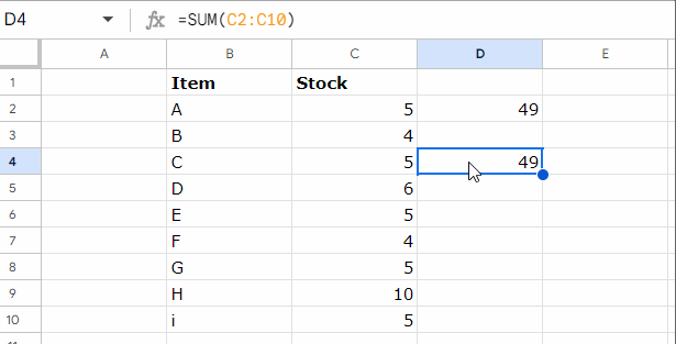
Direct reference: A1:C10
Indirect reference (text): "A1:C10"

To use a text string as a range, you wrap it with INDIRECT:

=SUM(A1:A10)
=SUM(INDIRECT("A1:A10"))

You can also store the range string in another cell:

If B1 contains A1:A10, then:
=SUM(INDIRECT(B1))

This approach is widely used to create dynamic ranges in Google Sheets.

Dynamic Indirect Range Example

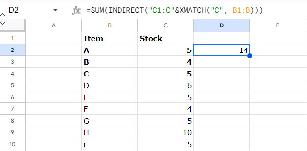
Suppose you want to sum values in column C up to the position of a value in column B.

Find the position using XMATCH:

=XMATCH("C", B1:B)

Build a dynamic range:

="C1:C"&XMATCH("C", B1:B)

Use INDIRECT:

=SUM(INDIRECT("C1:C"&XMATCH("C", B1:B)))

This creates a flexible, dynamic range based on lookup results.

SUM with INDIRECT and XMATCH totaling a dynamic range in Google Sheets

How to Highlight an Indirect Range in Google Sheets

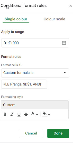
Use the following custom formula in Conditional Formatting:

=LET(r,SPLIT($D$1,":"),
AND(
  ISBETWEEN(ROW(),ROW(INDIRECT(INDEX(r,1))),ROW(INDIRECT(INDEX(r,2)))),
  ISBETWEEN(COLUMN(),COLUMN(INDIRECT(INDEX(r,1))),COLUMN(INDIRECT(INDEX(r,2))))
))

Highlighting an indirect range in Google Sheets using conditional formatting and a range string

Modify the Formula

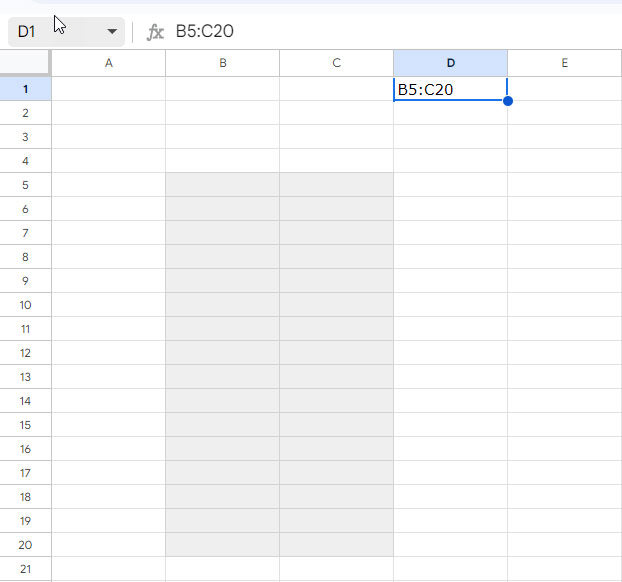
Replace $D$1 with the cell containing your range string
Or hardcode the range: "B5:C20"

Apply the Conditional Formatting Rule

Select your sheet range (e.g., B1:E1000)
Go to Format > Conditional formatting
Choose Custom formula is
Paste the formula
Pick a light fill color
Click Done

Applying custom formula rule in conditional formatting to highlight indirect range in Google Sheets

Tip: Keep the “Apply to range” as small as possible to improve performance.

How the Formula Works

The formula checks whether each cell falls within the indirect range using:

ROW() + ISBETWEEN → checks row boundaries
COLUMN() + ISBETWEEN → checks column boundaries
INDIRECT + SPLIT + INDEX → extracts the start and end references from the range string

The LET function improves readability by storing the range string once.

Practical Use Case

Use XLOOKUP + CELL to return the start and end addresses:

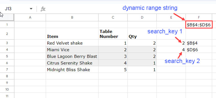
Using XLOOKUP and CELL to build a dynamic range string for highlighting in Google Sheets

=CELL("address", XLOOKUP(E3, $C$2:$C$7, $B$2:$B$7))
=CELL("address", XLOOKUP(E4, $C$2:$C$7, $D$2:$D$7))

Combine them into a range string (e.g., $B$4:$D$6):

=JOIN(":", F3:F4)

Feed that range string into the highlight formula.

This makes your highlighting fully dynamic.

Conclusion

This tutorial explains how to highlight an indirect range in Google Sheets using conditional formatting. It’s a practical workaround to visualize ranges used inside the INDIRECT function.

Want to dive deeper? Explore more conditional formatting techniques—from basic rules to advanced formula-driven setups—in the Ultimate Guide to Conditional Formatting in Google Sheets, where all related tutorials are organized in one place.