A dynamic H&V named range in Google Sheets automatically expands when you add values to the first row or column in the range.

For example, the current data range is A1:G20. When you add a value to cell A25, the range will become A1:G25. And when you add a value to cell K1, the range will become A1:K25. Also, it will adjust when you add or remove columns in the range.

The dynamic responsiveness of the formula we will use for this depends on the values in the topmost row and leftmost column of the range.

In short, this post describes how to create a fully dynamic named range in Google Sheets.

I have three separate formulas that answer the following questions:

1. How to create a dynamic named range with respect to row (vertical).
2. How to create a dynamic named range with respect to column (horizontal).
3. How to create a dynamic H&V named range (horizontal and vertical).

It is so simple to use these formulas, as you only need to specify two arguments: the first cell in the range and the sheet name of the range you use.

Create a Dynamic Named Range in Google Sheets with Respect to Row

Note: This is the vertical (V) part of the dynamic H&V named range in Google Sheets.

To create a dynamic vertical named range with respect to rows in Google Sheets, we need to specify two arguments in the formula.

• The cell reference of the first cell in the column where the data begins. This cell reference should be in text form, such as "B2".
• The sheet name.

For example, if your data starts in the cell Sheet1!B2, the first cell will be "B2" and the sheet name will be "Sheet1".

In the formula, we will use the names first_cell and sheet_name to represent the value expressions "B2" and "Sheet1", respectively.

Formula:

=LET(
     first_cell,"B2",
     sheet_name,"Sheet1",
     range,REGEXEXTRACT(first_cell,"[A-Z]"),
     sheet_name&"!"&first_cell&":"&range&
     XMATCH("?*",ARRAYFORMULA(TO_TEXT(INDIRECT(sheet_name&"!"&range&":"&range))),2,-1)
)

Steps

1. Enter the formula in any cell outside the column you want to use. As per the above example, you should use the formula outside column B. You can use this in a different sheet as well.
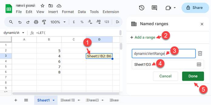
2. Go to the Data menu > Named ranges > Add a range.
3. In the Name field, enter dynamicVertRange.
4. In the Refers to the field, enter the cell reference of the cell that contains the formula, for example, Sheet1!D3. If you entered the formula in Sheet2!A1, use that cell reference instead.
5. Click Done.

We have created a dynamic named range with respect to rows. Because in this case, the rows are dynamic, not the columns.

How do we use it?

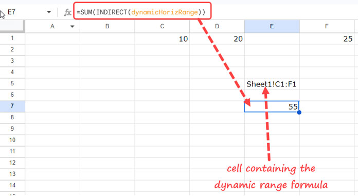
Unlike the named range, you should place double quotes around the dynamic named range. Then wrap it with the INDIRECT function. Here is an example of how to use it:

=INDIRECT("dynamicVertRange")

To sum up the data, you can use the following:

=SUM(INDIRECT("dynamicVertRange"))

To test whether it’s working, enter 10 in cell B9. The above formula will return 40.

Can I use this formula in Sheet2 or any sheet other than Sheet1? If so, what changes should I make?

Yes, you can use the above SUM formula as it is in any other sheet. You do not need to make any changes. This is applicable to any formula that you coded using the dynamic vertical range, which is INDIRECT("dynamicVertRange").

Create a Dynamic Named Range in Google Sheets with Respect to Column

Note: This is the horizontal (H) part of the dynamic H&V named range in Google Sheets.

To create a dynamic horizontal named range with respect to columns, we need to specify two arguments.

• The cell reference of the first cell in the row where the data begins. For example, "C1".
• The sheet name. For example, "Sheet1".

To further clarify, if your data starts in cell Sheet1!C1, the first cell will be "C1" and the sheet name will be "Sheet1".

In the formula, we will use the names first_cell and sheet_name to represent the value expressions "C1" and "Sheet1", respectively.

Formula:

=LET(
     first_cell,"C1",
     sheet_name,"Sheet1",
     range,REGEXREPLACE(first_cell,"[A-Z]",""),
     sheet_name&"!"&first_cell&":"&ADDRESS(ROW(INDIRECT(first_cell)),
     XMATCH("?*",INDEX(TO_TEXT(INDIRECT(sheet_name&"!"&JOIN(":",range,range)))),2,-1),4)
)

Enter this formula in any cell other than row 1, the row where we use to create the dynamic named range with respect to the column.

For example, enter the formula in cell E5 and create a named range that points to this cell from Data > Named ranges. You can use the name dynamicHorizRange for the range.

Similar to dynamicVertRange, dynamicHorizRange can be used in any sheet in the workbook.

How to Create a Dynamic H&V Named Range in Google Sheets

A dynamic H&V named range is responsive to both rows and columns. It’s two-dimensional. Therefore, it is important to be careful when placing the formula that is used to create the named range.

There are two approaches you can take:

1. Do not use the first column (A:A) and first row (1:1) for data entry. This means you can place the formula in cell A1. By default, the usable range will be B2:Z1000. You can add more rows at the bottom and more columns at the right.
2. If you want to use the full sheet for data entry, enter the formula in a different sheet.

In either case, the formula takes two parameters: the first cell of the range and the sheet name.

For example, the following formula creates a dynamic H&V named range that starts at cell C4 in Sheet1:

Formula:

=LET(
     first_cell,"C4",
     sheet_name,"Sheet1",
     rangeC,REGEXEXTRACT(first_cell,"[A-Z]"),
     rangeR,REGEXREPLACE(first_cell,"[A-Z]",""),
     sheet_name&"!"&first_cell&":"&ADDRESS(XMATCH("?*",
     INDEX(TO_TEXT(INDIRECT(sheet_name&"!"&rangeC&":"&rangeC))),2,-1),XMATCH("?*",
     INDEX(TO_TEXT(INDIRECT(sheet_name&"!"&JOIN(":",rangeR,rangeR)))),2,-1),4)
)

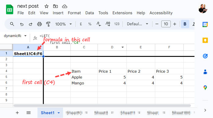
Enter the above formula in cell A1 and create a named range that points to cell A1. You can use the name dynamicRange to name the cell A1 within Data > Named ranges.

The named range in cell A1 will expand when you add values in the range C4:C or C4:4. It is responsive to the first row and column of the start cell, which is C4.

How is this useful?

Here are a few examples. I suggest you use them not in Sheet1.

To return the last column of a table dynamically, you can use the following CHOOSECOLS formula.

=CHOOSECOLS(INDIRECT(dynamicRange),-1)

Here is how to use the dynamic H&V named range within a FILTER formula.

=FILTER(INDIRECT(dynamicRange),CHOOSECOLS(INDIRECT(dynamicRange),1)="Apple")

This will return rows matching “Apple” in the first column of the range.

Conclusion

Named ranges are useful for creating cleaner formulas. Dynamic named ranges additionally bring flexibility to the range in use, as they expand when adding values in the first row (dynamicHorizRange), the first column (dynamicVertRange), or both (dynamicRange).