Conditional Format Duplicates Across Sheet Tabs in Google Sheets

Another detailed tutorial on how to identify duplicates in Google Sheets by highlighting. Let me shed some light on how to conditional format duplicates across sheet tabs in Google Sheets.

By saying ‘another tutorial’ I am just referring to one of my earlier tutorial that handles duplicates within one sheet tab. That contain some awesome tips and tricks.

Similar Topic: Highlight Duplicates in Single, Multiple Columns, All Cells in Google Sheets (within one sheet tab).

To conditional format duplicates across sheet tabs, I am going to use two functions. They are Countif and Indirect.

In conditional formatting rules, when you want to refer to a range in a different sheet tab, you must use the Indirect function.

Must Read: Role of Indirect Function in Conditional Formatting in Google Sheets.

Why are you using Countif?

The function Countif helps me to conditionally count a column. So if the Countif returns the count that’s more than 1, that means the criterion repeats.

Highlighting the cells wherever the Countif returns the value>1 is the logic in highlighting duplicates in Google Sheets.

To highlight duplicates across sheet tabs that within one Google Sheets file, as mentioned above, you must use the function Indirect and multiple Countif formulas.

Let’s see how all that formulas develop.

Highlight/Conditional Format Duplicates Across Sheet Tabs in Google Sheets

To make the formulas simple to you, I am only using two sheet tabs in my example. So please do carefully follow my example and that can help you to extend the formulas for more sheets.

The Formula to Highlight Duplicates Across Sheet Tabs – Single Column

Here is the content in my column A in Sheet1.

Sheet1:

duplicates across sheets - data in Sheet 1

See what happens in Sheet2 when I enter duplicates of Sheet1 column 1 values.

Sheet2:

highlight duplicates across sheets

Just go back to Sheet1 and see that the duplicates highlighted there too.

The formula to Conditionally Format Duplicates Across Sheet Tabs in Single Column:

For Sheet1:

=(countif($A$2:$A,A2)+countif(indirect("Sheet2!$A$2:$A"),A2))>1

For Sheet2:

=(countif($A$2:$A,A2)+countif(indirect("Sheet1!$A$2:$A"),A2))>1

I have already explained to you how this formula highlights duplicates in different sheet tabs.

Are you new to Google Sheets? If yes, then follow the below instructions to apply this custom rule.

The conditional formatting is available under the menu Format in Google Doc Sheets.

Steps to Conditional Format Duplicates:

1. Select the range A2: A in Sheet1.

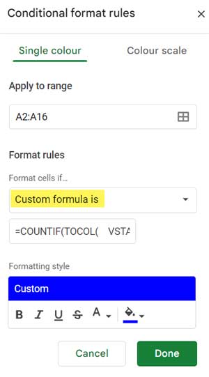
2. Open the conditional format rule from the menu Format > Conditional Format.

Apply the above first formula there as below.

conditional format rule to highlight repeating values

In Sheet2 also follow the above same instructions.

The Formula to Conditional Format Duplicates Across Sheet Tabs – Two Columns

Honestly, I don’t know how to explain this scenario correctly. So I am depending screenshots.

Here my sheets that involved in highlighting duplicates across sheet tabs are Sheet3 and Sheet4.

The Values in Sheet3:

two column duplicates in two sheets - Sheet 3

The Values in Sheet4:

two column duplicates in two sheets - Sheet 4

See the highlighting pattern. If values in column A and Colum B match in the same sheet or in a different sheet more than once, such rows are duplicates and subsequently got highlighted.

Here are the formulas to highlight duplicates across sheet tabs in two columns:

The Formula for Sheet3:

=(countifs($A$2:$A,$A$2:$A,$B$2:$B,$B$2:$B)+countifs(indirect("Sheet4!$A$2:$A"),$A$2:$A,indirect("Sheet4!$B$2:$B"),$B$2:$B))>1

Select the range A2: B in Sheet3 and apply this conditional format rule.

The Formula for Sheet4:

=(countifs($A$2:$A,$A$2:$A,$B$2:$B,$B$2:$B)+countifs(indirect("Sheet3!$A$2:$A"),$A$2:$A,indirect("Sheet3!$B$2:$B"),$B$2:$B))>1

Select the range A2: B in Sheet4 and apply this rule.

Similarly, you can add more columns and more sheets. That’s all.

Follow the above examples to conditional format duplicates across sheets in Google Sheets. Enjoy!

Copy Formatted Sheet

20 COMMENTS

Dannielle February 12, 2022 At 5:25 am

Hello! It has been helpful! I am wondering how I would do this:

Sheet 2 column A has IDs.
Sheet 1 column A has IDs, and column B has a “Yes” or “No” answer.

I want to highlight Sheet 2, column A if column B in Sheet 1 (with the matching ID number) = “Yes.”

I do hope that made sense and that you can help!

Thank you!

- Prashanth February 12, 2022 At 9:40 am
  
  Hi, Dannielle,
  
  Try this rule in Sheet2!A2:A1000.
  
  =ifna(vlookup(A2,indirect("Sheet1!A2:B1000"),2,0))="Yes"
  
Jj S. July 19, 2021 At 11:53 am

Very helpful, thank you!!

Divya June 8, 2021 At 1:20 am

Can we highlight duplicates in multiple sheets within a workbook in google sheets?

Can you write the syntax for 6 sheets?

- Prashanth June 8, 2021 At 10:11 am
  
  Hi, Divya,
  
  I don’t recommend highlighting duplicates across several sheets as it can affect performance.
  In that case, I would recommend importing data to a single sheet and then highlight it.
  
  Query Syntax/formula to Import cell range A2:A in three sheets to the fourth sheet in that workbook:
  
  =Query({Sheet1!A2:A;Sheet2!A2:A;Sheet3!A2:A}, "Select * where Col1 is not null")
  
  If you are still interested in highlighting across six sheets, here is the syntax that you can follow.
  
  For two sheets, I have already explained. Here is when three sheets are involved.
  
  Format “Apply to range” is A2:A in all three sheets (tabs).
  
  Sheet 1:
  
  =(countif($A$2:$A,A2)+countif(indirect("Sheet2!$A$2:$A"),A2)+ countif(indirect("Sheet3!$A$2:$A"),A2))>1
  
  Sheet2:
  
  =(countif($A$2:$A,A2)+countif(indirect("Sheet1!$A$2:$A"),A2)+ countif(indirect("Sheet3!$A$2:$A"),A2))>1
  
  Sheet 3:
  
  =(countif($A$2:$A,A2)+countif(indirect("Sheet1!$A$2:$A"),A2)+ countif(indirect("Sheet2!$A$2:$A"),A2))>1
  
  You can follow this pattern to include more sheets in the conditional format rule.
  
Lee April 1, 2021 At 8:57 am

Hi Prashanth,

Great resource, I keep coming back but slowly getting it. Sorry, I’m new to spreadsheets.

Can you show me a formula to remove duplicates across a multiple 7 to 31 across tabs in Google sheet (each day in month list)?

I’ve seen the 2 videos, and it didn’t work for me sorry 🙁

I’d like to check 7 days period.

Ang March 26, 2021 At 1:29 am

This is just what I’m looking for, though what would the formula be for Sheet 2 if I do not want to highlight duplicates that are within Sheet 2?

If I list Avacaods twice within Sheet 2 they are both highlighted as duplicates (Avacados are not listed in Sheet 1).

I only want to highlight duplicates comparing to Sheet 1.

- Prashanth March 26, 2021 At 5:53 pm
  
  Hi, Ang,
  
  Replace the Sheet2 highlighting rule (formula) with the below one.
  
  =countif(indirect("Sheet1!$A$2:$A"),A2)>0
  
F October 6, 2020 At 11:39 pm

Thanks for this solution!

For Sheet1:

=(countif($A$2:$A,A2)+countif(indirect("Sheet2!$A$2:$A"),A2))>1

For Sheet2:

=(countif($A$2:$A,A2)+countif(indirect("Sheet1!$A$2:$A"),A2))>1

How can we add the same formula if we have sheet 3, sheet 4, sheet x …

Thank you!

Donna June 23, 2020 At 8:48 am

This is very helpful. I need to check if a value in a cell exists in a column in another worksheet. How to make this formula work in that situation?

Thanks!

- Prashanth June 24, 2020 At 8:38 am
  
  Hi, Donna,
  
  You may use the MATCH function.
  
  To match the value in cell B4 (“Sheet1”) in another sheet (column C in “Sheet2”) use the below formula in cell C4 in “Sheet1”.
  
  =ifna(match(B4,Sheet2!C:C)>0,FALSE)
  
  It would return TRUE for match and FALSE for a mismatch.
  
janine April 11, 2020 At 11:54 pm

Hi, whoa I can never figure these things out myself! I was wondering if you could help me – I have two lists of customers

A: All customers (including refunds)
B: All refunds.

So what I’m trying to do …. is produce a sheet that ONLY shows customers who did not get a refund. Using your strategy above works….except now the rows are highlighted for me to see but I can’t bulk delete them…

Is there a way to do something like…
IF THERE ARE DUPLICATES, DELETE BOTH?

I can upload both lists on the same sheet, it doesn’t have to be separate sheets so I think that will make it easier?

But everything I’ve looked online only shows me how to delete duplicates. What I’m trying to do is actually DELETE both when duplicates are found.

any insight you can provide, I would really appreciate!

- Prashanth April 12, 2020 At 11:10 am
  
  Hi, janine,
  
  If you use conditional formatting, now you can bulk delete the highlighted cells. I hope you are aware of the new feature in Sheets – Filter or Sort by Font or Cell Color in Google Sheets.
  
  If you are looking to filter the customers who didn’t get a refund, then try this filter.
  
  A1:A – All customers (including refunds)
  B1:B – All refunds.
  
  Assume the first row (A1:B1) contains headers.
  
  The formula to be used in cell C2 (case insensitive):
  
  =filter(A2:A,countif(B2:B,A2:A)=0)
  
  Case sensitive formula:
  
  =filter(A2:A,regexmatch(A2:A,"^"&textjoin("$|^",true,B2:B)&"$")=FALSE)
  
Agam Singh December 26, 2018 At 10:08 am

This is so useful! Thank you so much!

Would you be able to suggest a solution where this also works if cells in some of the columns are empty? As it stands today, the above does not highlight rows that have blank cells (even if they are identical).

As an example use case, when importing bank statements from a “new” sheet to an “existing” sheet, we want to highlight duplicate rows, but for two of the columns (debit and credit), there are values only in one of those columns.

Example data:
Date, Description, Debit, Credit
====================
01/01, Target, $10, <>
01/01, BestBuy returns,<>, $50
02/01, Target, $20, <>

Your help would be much appreciated. Thank you once again.

- Prashanth December 26, 2018 At 11:24 am
  
  Hi, Agam Singh,
  
  Please share a demo sheet and manually highlight the cell/cells (your desired result). Then I can possibly try.
  
Sebastian October 1, 2018 At 5:21 pm

Hi,

can I use match function across two tabs? I used COUNTIF, but the problem is that it highlights not only the duplicates between the tabs but also duplicates in one tab.

Best,
Sebastian

- Prashanth October 1, 2018 At 5:38 pm
  
  Hi, Sebastian,
  
  Yes! You can use. But don’t forget to use INDIRECT as it’s a must in conditional formatting to refer to another tab.
  
  I have a new tutorial but that also using COUNTIF.
  
  Highlight Matches or Differences in Two Lists in Google Sheets
  
  - Sebastian October 1, 2018 At 5:46 pm
    
    Hi Prashanth,
    
    Exactly, I used the Countif but do not know how to do it with a Match. Could you write it for me, please?
    
    - Prashanth October 1, 2018 At 5:54 pm
      
      Hi,
      I’ll try. Please make a ‘demo’ Sheet and share it with me. In that sheet clearly mention the output that you expect.
      Thanks.
      
      - Sebastian October 3, 2018 At 7:56 pm
        
        Hi Prashanth,
        Thanks, I used countif formula but without taking into consideration one tab and it works. Thank you again. You are doing a great job with this blog.