Highlighting duplicates in Google Sheets helps you quickly identify repeated values in your data. Whether you are working with a single column, entire rows, or a full dataset, conditional formatting makes this task simple and efficient.

In this tutorial, we will use the COUNTIF and COUNTIFS functions to highlight duplicates in different scenarios in Google Sheets.

Quick Answer: Highlight Duplicates in Google Sheets

Use this formula in Conditional Formatting to highlight duplicates in a column:

=COUNTIF($A$1:$A, A1)>1

This method works for both small datasets and large spreadsheets.

Example 1: Highlight Duplicates in a Single Column

When you want to highlight duplicates in a single column, follow these steps. There are two highlighting options available:

1. The first option highlights all occurrences of duplicates.
2. The second option highlights duplicates excluding the first occurrence.

For example, let’s consider values in column A, starting from cell A1.

To highlight all occurrences of duplicates in column A starting from A1, use the formula:

=COUNTIF($A$1:$A, A1)>1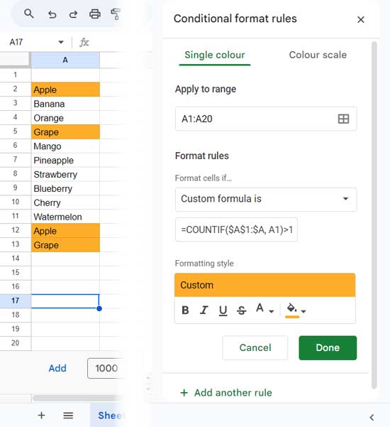

If you want to apply this rule starting from cell A10 in column A, adjust the formula to: =COUNTIF($A$10:$A, A10) > 1

Ensure that the “Apply to range” in Conditional Formatting matches the starting range specified in the formula (e.g., A1:A or A10:A).

Here’s how to set it up:

1. Select the range (e.g., A1:A).
2. Click on “Format” > “Conditional formatting”.
3. If there’s already a rule applied, click “Add another rule” in the sidebar panel.
4. Under “Apply to range”, enter the correct range (e.g., A1:A or A10:A).
5. Choose “Custom formula is” under “Format rules” and enter the respective formula.
6. Select your desired formatting style and click “OK”.

To highlight duplicates from the second occurrence onwards, use the formula:

=COUNTIF($A$1:$A1, A1)>1

Example 2: Highlight Duplicate Rows in Google Sheets

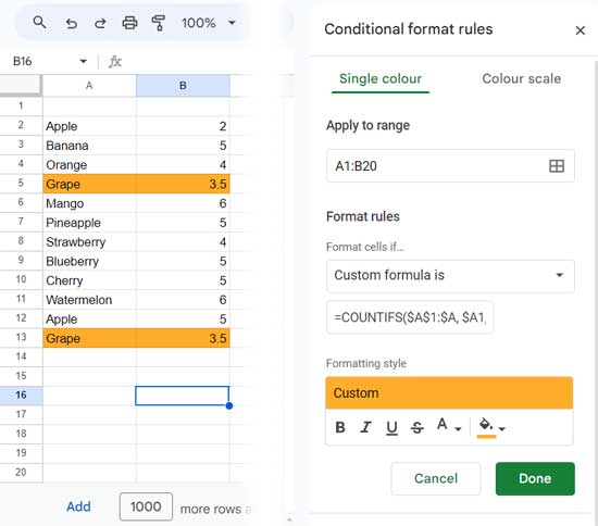
Highlighting duplicates row-wise differs from highlighting duplicates in a single column. Here, we evaluate the entire row (within the selected range) as a single unit.

For example, if A1:B1 contains “Apple” and “Grade A”, and A2:B2 contains the same values, they are duplicates. However, if B2 contains “Grade B”, the two rows are not duplicates.

Here, use the COUNTIFS formulas based on your requirement, i.e., whether you want to highlight all duplicate rows or duplicates from the second instance onwards.

To highlight all occurrences of duplicate rows for the range (Apply to range) A1:B, use the following formula:

=COUNTIFS($A$1:$A, $A1, $B$1:$B, $B1)>1

If you have more columns, include them in the formula accordingly.

To highlight duplicate rows from the second instance onwards, use:

=COUNTIFS($A$1:$A1, $A1, $B$1:$B1, $B1)>1

Example 3: Highlight Duplicates Across the Entire Sheet

Some of you might want to highlight duplicates if they appear anywhere in a sheet. For example, if you want to highlight duplicates in the range B2:D, use the following formula:

=COUNTIF($B$2:$D, B2)>1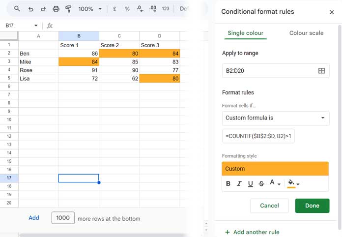

Use this rule to highlight duplicates across the entire sheet.

Please note that the “Apply to range” setting is important. When you apply the formulas to different ranges, you should modify them accordingly.

Additional Tips

Here I’ll show you how to use some of the above formulas in a slightly different way in real-life examples.

Highlight Frequently Purchased Items (Monthly)

Here, we have the date of purchase in column A and the item name in column B, with the Apply to range set to A1:B. You can use the following formulas:

• To highlight all occurrences of duplicates:

=ArrayFormula(COUNTIFS(EOMONTH($A$1:$A, 0), EOMONTH($A1, 0), $B$1:$B, $B1)>1)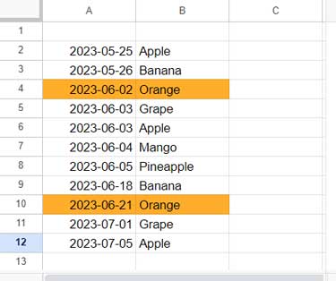

• For highlighting only from the second occurrence of duplicates:

=ArrayFormula(COUNTIFS(EOMONTH($A$1:$A1, 0), EOMONTH($A1, 0), $B$1:$B1, $B1)>1)

In addition to the COUNTIFS function, we use the EOMONTH function, which converts the dates to the end-of-the-month dates. This ensures that, for each month, there is one unique date.

We need to use the ARRAYFORMULA function since we are applying a non-array function (EOMONTH) within an array context.

These two formulas are derived from our example 2, “Highlight Duplicates by Row.” The only additions here are the ARRAYFORMULA and EOMONTH functions.

Highlight Frequently Purchased Items (Daily)

Here, you can use the same formulas as under “Highlight Duplicates by Row.” No changes are necessary unless you have timestamps instead of dates.

If you have timestamps, use the INT function along with ARRAYFORMULA. For example, if A1:A contains timestamps and B1:B contains items, use the following formula:

• To highlight all occurrences of duplicates:

=ArrayFormula(COUNTIFS(INT($A$1:$A), INT($A1), $B$1:$B, $B1)>1)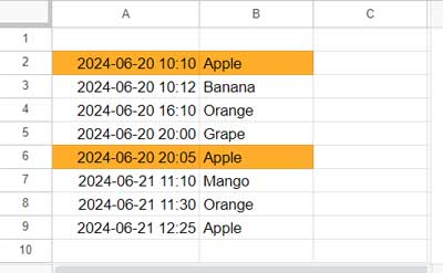

• For highlighting only from the second occurrence of duplicates:

=ArrayFormula(COUNTIFS(INT($A$1:$A1), INT($A1), $B$1:$B1, $B1)>1)

Conclusion

You can easily highlight duplicates in Google Sheets using conditional formatting with COUNTIF or COUNTIFS. Whether you are working with a single column, entire rows, or full datasets, these formulas help you quickly identify repeated values.

This tutorial is part of The Ultimate Guide to Conditional Formatting in Google Sheets, where you can explore many more formatting techniques and examples.

Resources

Here are a few related tutorials on highlighting duplicates in Google Sheets:

• Highlight Partial Matching Duplicates in Google Sheets
• Highlight Visible Duplicates in Google Sheets
• How to Conditional Format Duplicates Across Sheet Tabs in Google Sheets