We can make duplicates to unique in Google Sheets by assigning alphabets, roman letters or numbers in sequential order. Let’s see how?
For example, if the string “apple” occurs thrice, we can make it unique by adding roman numbers to it as below.
apple
apple_I
apple_II
For this, we require a combination of three formulas. They are running count, autofill sequential roman/alphabets/numbers and Vlookup.
We can use these formulas individually and these formulas are not much complicated as you think.
So first I will use these formulas in their own columns (helper columns) to make duplicates to unique in Google Sheets. Then we can learn how to combine all these formulas in a flash to avoid helper columns.
Here is an example of making duplicates to unique by assigning occurrence numbers (alphabets/numbers/roman letters) in Google Sheets.
Screenshot # 1:
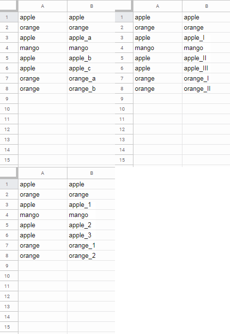
You have the flexibility to choose which character to use to make duplicates to unique. I mean you can switch between roman letters, numbers or alphabets.
In the above example, there are duplicates in column A. Let’s consider the item “apple”.
The formula adds occurrence number I (1 or a) to the second occurrence of the item “apple”, II (2 or b) to the third occurrence of the same item and so on.
Let’s see how to make duplicate values in a column to unique by assigning occurrence numbers/letters as explained above in Google Sheets.
Three Formulas to Add Occurrences to Duplicates in Google Sheets
Step 1: Formula in ‘Test’ Tab
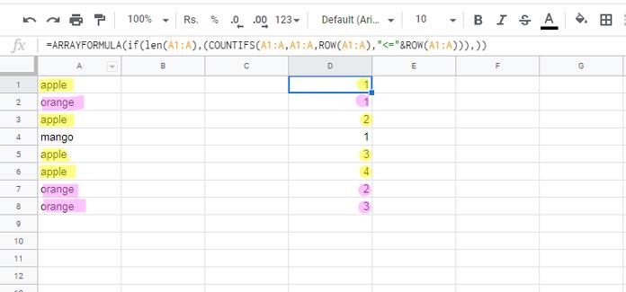
The sample data used in the above screenshot is in the tab named ‘Test’. In that tab, in cell D1 enter the following running count formula.
=ARRAYFORMULA(if(len(A1:A),(COUNTIFS(A1:A,A1:A,ROW(A1:A),"<="&ROW(A1:A))),))For this formula explanation, please refer to this page – Running Count in Google Sheets – Formula Examples.
I have the comfort of leaving the running count explanation as I have already explained it 🙂
Screenshot # 2:
Step 2: Formulas in ‘Test_1’ Tab (Populating Sequential Roman | Alphabets | Numbers)
Please scroll up and again watch the live/animated screenshot # 1 (GIF).
What we want to do is to make duplicates to unique in Google Sheets by assigning characters.
Here ‘characters’ can be sequential numbers/alphabets or roman numbers. Let me call it occurrence types. I am going to give you options to switch between the occurrence types.
Note: I am only considering 50 duplicates of each value. If you want more than that, you may change the below formulas accordingly (as instructed below).
Four Formulas in Test_1 Tab
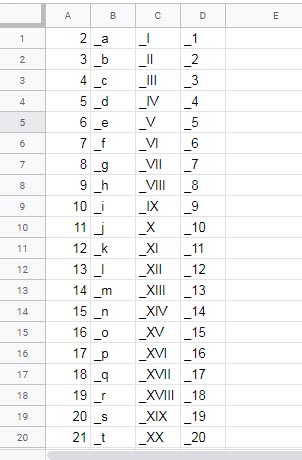
In cell A1, use the following formula.
=ArrayFormula(row(A2:A51))Change A51 to A101 to include 100 duplicates of each value.
This formula would return sequential numbers from 2 to 51 in the range A1:A50. It’s an array formula so it will expand from A1 to A50 automatically.
Formula Explanation – Auto Serial Numbering in Google Sheets with Row Function.
In cell B1, insert the below formula and drag it to B50 (or B100 for 100 duplicates) to fill alphabets (lowercase letters).
="_"&lower(regexreplace(address(1,row(B1)),"[^A-Z]",""))The formula will also add an underscore character as the prefix value to the alphabets (please see the screenshot # 3 below).
The "_"& part at the beginning of the formula handles this. The rest of the formula part detailed here – How to Autofill Alphabets in Google Sheets.
In cell C1, use the following formula to populate roman numbers. These numbers will also use the underscore prefix.
=ArrayFormula("_"&ROMAN(row(B1:B50)))The above is also an array formula. Change B50 to B100 for 100 duplicates.
Related: How to Use Roman Numbers in Google Sheets.
In cell D1, repeat the A1 formula. But this time the range must be A1:A50 (A100 for 100 duplicates) and we must add an underscore prefix. Here is that formula.
=ArrayFormula("_"&row(A1:A50))Screenshot # 3:
Now the final formula in the ‘Test’ tab that will make duplicate values to unique values by assigning their sequence in Google Sheets.
Step 3: Formula in ‘Test’ Tab – Make Duplicates to Unique in Google Sheets Using Vlookup
We can connect all the above formulas using Vlookup. That will make duplicates to unique.
Formula:
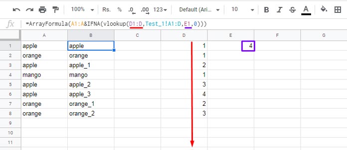
=ArrayFormula(A1:A&IFNA(vlookup(D1:D,Test_1!A1:D,E1,0)))The above Vlookup formula is in cell B1 in the ‘Test’ tab.
Screenshot # 4:
What’s the role of the Vlookup to make duplicates to unique in Google Sheets?
Vlookup searches down the running count, i.e. values in D1:D in the ‘Test’ tab (screenshot # 4), in the first column of the range A1:D in the ‘Test_1’ tab (screenshot # 3).
Then it would return the values from columns 2, 3 or 4 from the ‘Test_1’ tab based on the input in cell E1 in the ‘Test’ tab (screenshot # 4).
That means if you type 2 in cell E1, it would return alphabets, 3 would return roman numbers and 4 will return (Arabic) numbers.
The values in column A has been then combined with the Vlookup output using A1:A& (at the beginning of the Vlookup).
I just don’t want to use the helper columns/tabs and multiple formulas. Can you combine the above formulas and make duplicates to unique in Google sheets?
Yes! Here is the step by step instructions.
Combination Formula to Add Sequence Numbers to Duplicates in Google Sheets
By changing the cell/array reference with corresponding formulas in the Vlookup above, we can make a single formula to make duplicates to unique in Google Sheets. Here are the steps.
Step 1: Replace the Vlookup Range with Virtual Range (Sequence)
In the above Vlookup, the range is Test_1!A1:D. Replace that with {row(A2:A51),"_"&ROMAN(row(B1:B50))}.
The latter formula combines ‘Test_1’ column A and C values as a two-column array.
We can only combine cell A1 formula with cell C1 or cell D1 formula to form an array. We can’t use the formula in cell B1 from that tab (alphabets), as it is a non-array formula.
So the formula will be;
=ArrayFormula(A1:A&IFNA(vlookup(D1:D,{row(A2:A51),"_"&ROMAN(row(B1:B50))},E1,0)))
or
=ArrayFormula(A1:A&IFNA(vlookup(D1:D,{row(A2:A51),"_"&row(A1:A50)},E1,0)))
In the above two, I am preferring the first one (roman numbers) and so using it.
Step 2: Replace the Vlookup Search Key with Virtual Range (Occurrence)
The Vlookup search key range is D1:D in the ‘Test’ tab.
We can replace D1:D with corresponding formula, i.e. if(len(A1:A),(COUNTIFS(A1:A,A1:A,ROW(A1:A),"<="&ROW(A1:A))),) from cell D1.
=ArrayFormula(A1:A&IFNA(vlookup(if(len(A1:A),(COUNTIFS(A1:A,A1:A,ROW(A1:A),"<="&ROW(A1:A))),),{row(A2:A51),"_"&ROMAN(row(B1:B50))},E1,0)))Then replace E1 with 2 as there are only two columns in the Vlookup range. See the final Vlookup below.
Step 3: Combination Formula to Make Duplicates to Unique by Assigning Sequence Nos in Google Sheets
Key the below complex Vlookup in cell B1.
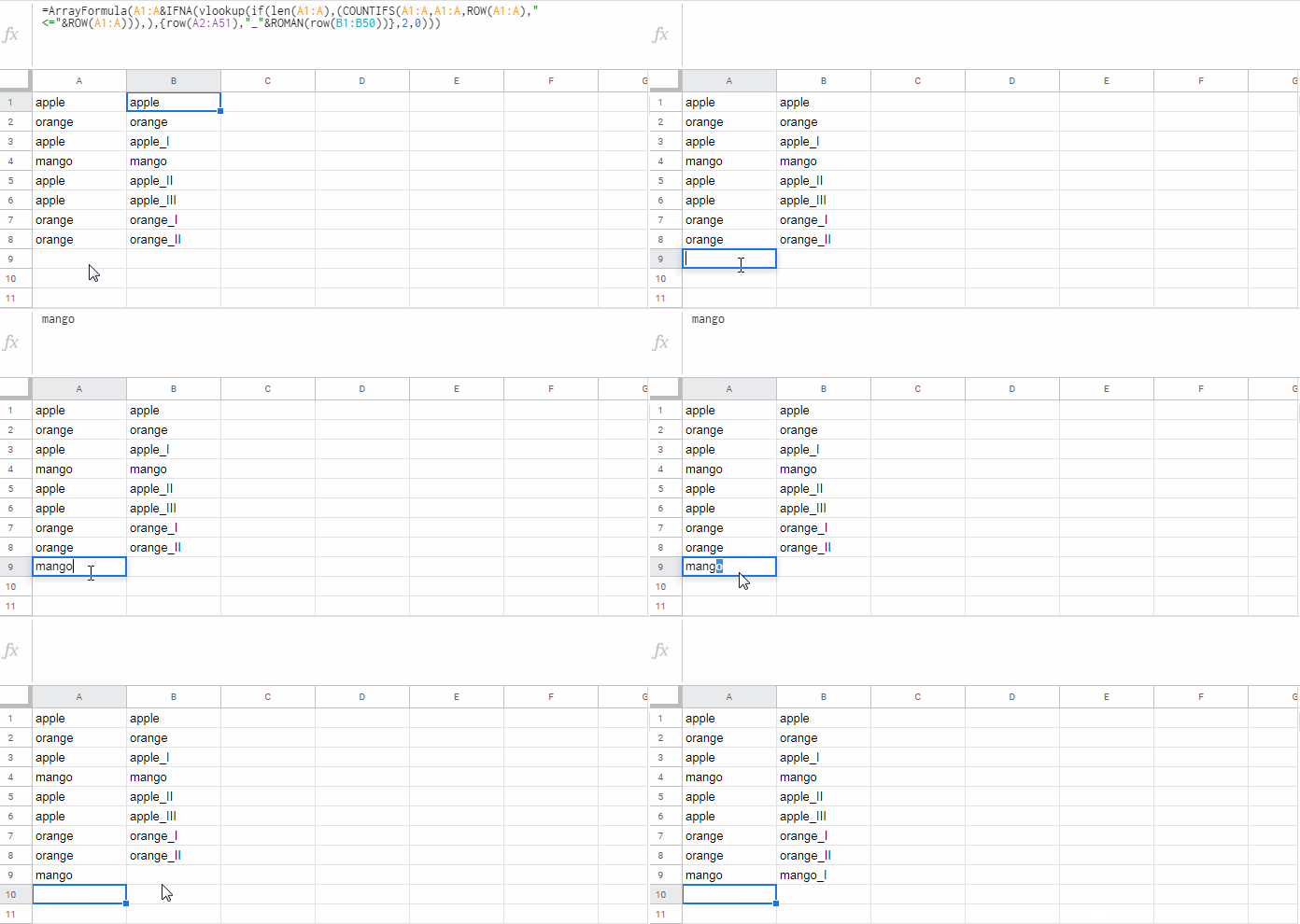
=ArrayFormula(A1:A&IFNA(vlookup(if(len(A1:A),(COUNTIFS(A1:A,A1:A,ROW(A1:A),"<="&ROW(A1:A))),),{row(A2:A51),"_"&ROMAN(row(B1:B50))},2,0)))Feel free to delete the ‘Test_1’ tab and the formula in cell D1 in the ‘Test’ tab and the value in cell E1 in the same tab.
Screenshot # 5:
That’s all. Enjoy!


