In this tutorial, you’ll learn how to use Roman numerals in Google Sheets. Additionally, I’ll answer the following questions related to Roman numbering in Google Sheets:
- How to auto-generate Roman numerals as serial numbers.
- How to convert any number from 1 to 3999 into Roman numerals using the ROMAN function.
- How to convert Roman numerals back to Arabic numbers using the ARABIC function.
To answer all of these questions, I’ll first introduce the two functions mentioned above. Let’s begin with how to use Roman numerals in Google Sheets.
ROMAN Function – Syntax and Examples
In the following syntax, the argument rule_relaxation is optional. With rule relaxation, you can shorten the representation of Roman numerals to some extent by applying relaxed rules to the traditional syntax. You can specify values from 0 to 4 for rule relaxation, where 0 is the default and represents the correct and traditional way to write Roman numerals.
Syntax:
ROMAN(number, [rule_relaxation])Examples:
=ROMAN(499)// returns CDXCIX=ROMAN(499, 1)// returns LDVLIV=ROMAN(499, 2)// returns XDIX=ROMAN(499, 3)// returns VDIV=ROMAN(499, 4)// returns ID
Regarding rule relaxation, let’s consider the first two Roman numerals, “CDXCIX” and “ID”:
CDXCIX:
- CD: 500 – 100 = 400
- XC: 100 – 10 = 90
- IX: 10 – 1 = 9
So, CDXCIX = 400 + 90 + 9 = 499.
ID:
- 500 – 1 = 499.
Please note that the ROMAN function is capable of formatting numbers from 1 to 3999, inclusive.
For more information on rule relaxation, please check out this source: Official Documentation
ARABIC Function – Syntax and Examples
In Google Sheets, you can use the ARABIC function to compute the value of Roman numerals ranging from 1 to 3999.
Syntax:
ARABIC(roman_numeral)Example:
The following formulas will return 499, even though the Roman numerals are in a rule-relaxed format:
=ARABIC("CDXCIX")=ARABIC("LDVLIV")=ARABIC("XDIX")=ARABIC("VDIV")=ARABIC("ID")
Now it’s time to explore some practical examples of using the ROMAN and ARABIC functions.
Auto-generate ROMAN Numerals as Serial Numbers
Want to use Roman numerals as serial numbers in a column or row? You can use SEQUENCE within ROMAN and enter the formula as an array formula.
The following formula will return the Roman numerals from 1 to 100 in a column:
=ArrayFormula(ROMAN(SEQUENCE(100)))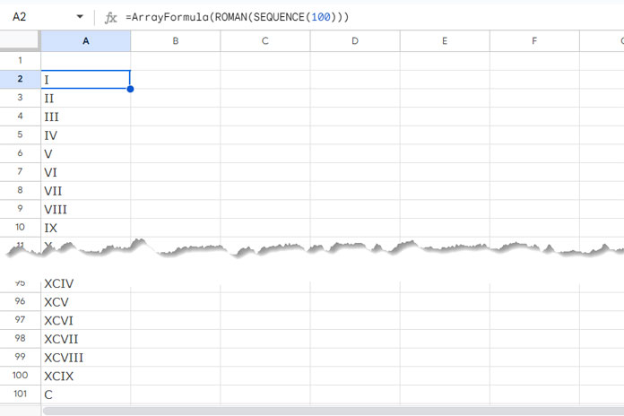
If you want them in a row, use this formula:
=ArrayFormula(ROMAN(SEQUENCE(1, 100)))You can replace 100 with any number between 1 and 3999 in the above formulas to generate Roman serial numbers accordingly.
How to Convert Roman Numerals to Arabic Numbers
You can use the ARABIC function to convert any Roman numeral back to an Arabic number. However, if you type the formula like this, it won’t work:
=ARABIC(IV)Instead, the correct formula would be:
=ARABIC("IV")The Roman numeral should be enclosed in double quotes, just like text. Alternatively, you can enter the Roman numeral in a cell and reference that cell in the ARABIC function.
How to Use Roman Numerals in Arithmetic Operations in Google Sheets
Assume you have the Roman numeral IV and want to add I to it to get V. How do you do that?
To use Roman numerals in calculations, you should convert them to Arabic numerals:
=ROMAN(ARABIC("IV") + ARABIC("I"))The above formula will add IV + I and return V.
Error Handling
The ROMAN function will return the #VALUE! error when the specified number is not between 1 and 3999. You can wrap the formula with IFERROR to handle this error.
If you want to inform the user of the specific reason for the error, you can apply a logical test as follows:
=IF(ISBETWEEN(A1, 1, 3999), ROMAN(A1), IF(ISTEXT(A1), "Invalid Input: Text Not Supported", IF(OR(A1<1, A1>3999), "Error: Number should be between 1 and 3999",)))The ARABIC function will return a similar error if the specified value is not a valid Roman numeral or if it is text. To remove that error, simply wrap it with IFERROR.


