IFERROR and IFNA are two Google Sheets functions that can be used to remove errors and return a custom value. IFNA is specifically for NA() errors.

In this tutorial, we will discuss everything about the IFERROR function, which is a powerful tool but can also be misused if used too liberally. We will discuss when to use IFERROR and when to avoid it.

Syntax and Arguments

Syntax:

IFERROR(value, [value_if_error])

Arguments:

• value: The value that the function will check for an error. If value is not an error, the function will return value.
• value_if_error: (Optional) The value that the function will return if value is an error. If value_if_error is omitted, the function will return an empty string.

How to Use the IFERROR Function in Google Sheets

Here are some examples of how to use the IFERROR function:

Basic Formula

Cell A1 contains 4500 and B1 contains 0. The following formulas will return #DIV/0! error because the divisor is zero.

=A1/B1
=DIVIDE(A1,B1)

We can remove that error using Google Sheets IFERROR function as follows:

When you want to return blank:

=IFERROR(A1/B1) // returns blank or the result of A1/B1
=IFERROR(DIVIDE(A1,B1)) // returns blank or the result of DIVIDE(A1,B1)

When you want to return a custom value:

=IFERROR(A1/B1,0) // returns zero or the result of A1/B1
=IFERROR(DIVIDE(A1,B1),0) // returns zero or the result of DIVIDE(A1,B1)

Example of Using the IFERROR Function in an Array Formula

In the following example, to find the unit rates of products using an array formula, we can use the following formula:

=ArrayFormula(IFERROR(J3:J/C3:C))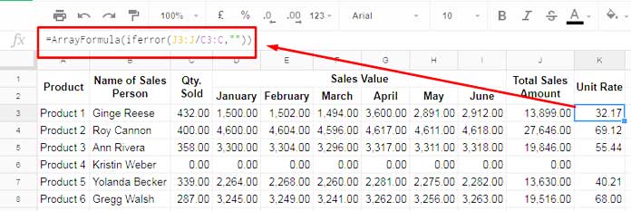

This formula will return the unit rates of products in column K, but will avoid the DIV/0! error if columns J and C are blank or contain zero, or if column J contains zero.

Here is a breakdown of the formula:

• The ArrayFormula function applies the formula to all of the cells in the specified range.
• The IFERROR function checks for errors and returns a custom value if an error is found. In this case, the custom value is an empty string.
• J3:J/C3:C: This divides the values in cells J3:J by the values in cells C3:C.

Google Sheets IFERROR Function Formatting Issue With ArrayFormula (Explained)

If you wrap a currency-formatted formula in the IFERROR function, the formatting may be lost. For example, the following formula will return the currency formatting in the result:

=ArrayFormula(B4:B8*C4:C8)

But this formula, which uses the IFERROR function, will not:

=ArrayFormula(IFERROR(B4:B8*C4:C8))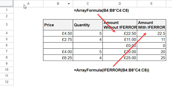

To fix the formatting issue, you can:

• Select the result and apply the currency formatting manually by clicking Format > Number > Currency.
• Use the TO_DOLLARS function with IFERROR. For example, the following formula will return the ‘default’ currency formatting in the result:

=ArrayFormula(TO_DOLLARS(IFERROR(B4:B8*C4:C8)))

Similar functions for date and percentage:

There are two similar functions that you can use when you want to retain date and percentage formatting:

• TO_DATE
• TO_PERCENT

Example:

The following formula will return the end-of-month dates and will retain the default date formatting in the result.

=ArrayFormula(TO_DATE(IFERROR(EOMONTH(DATEVALUE(A3:A),0))))

When to Use and Not Use the IFERROR

The IFERROR function can be a very useful tool for handling formula errors. However, it is important to use it carefully.

In some cases, it is important to understand why a formula is returning an error so that you can fix the problem.

For example, if an XLOOKUP function is returning an #N/A error, it is important to check that the search key is correct and that the data in the lookup range is valid.

If you simply wrap the XLOOKUP function in the IFERROR function, you may mask the underlying problem.

As a general rule, you should only use the Google Sheets IFERROR function to handle formula errors that you cannot prevent.

For example, if you are using an XLOOKUP or VLOOKUP function to search for a customer’s name in a database, you cannot prevent the formula from returning an #N/A error if the customer’s name is not in the database. However, you can use IFERROR to handle the error and return a more informative message to the user.