If you work with category-wise data in Google Sheets, you’ve probably faced the need to assign serial numbers that reset based on a group — for example, numbering items by category, sub-category, or any other subgroup. This process is called Group-Wise Dependent Serial Numbering in Google Sheets.
Understanding this concept is crucial because there are two common ways to interpret it, and the approach you choose depends on your reporting or analysis needs.
Two Approaches to Group-Wise Dependent Serial Numbers
1. Row-wise Dependent Serial Numbering
In this approach, the serial number increments for every row within a subgroup.

Explanation:
- The Dependent Serial No. resets for each Product + Category.
- It increments for every row within that subgroup.
2. Sub-Category-Based Dependent Serial Numbering
Here, the serial number remains the same for all rows in a subgroup and increments only when the subgroup changes.
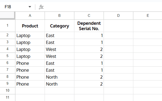
Explanation:
- The Dependent Serial No. resets per Product.
- All rows in the same Category share the same number.
- It increments only when the Category changes within the same Product.
Key Difference at a Glance
The Dependent Serial No. may either increment per row within a group or remain the same for all rows in a sub-group, depending on your numbering logic.
Formulas for Group-Wise Dependent Serial Numbering in Google Sheets
Now that we’ve seen the differences, let’s dive into the formulas you can use to implement both methods.
Note:
The best approach is to use sorted data when applying Group-Wise Dependent Serial Numbering. While the formulas will still work with unsorted data, any repeated groups appearing later in the dataset may be treated as a continuation of the earlier group rather than a new group. Sorting ensures that each group is recognized correctly and the dependent serial numbers reset as intended.
1. Row-wise Dependent Serial Number Formula
Row-wise dependent serial numbering is fairly simple. It’s essentially the running occurrence of Product and Category. For the sample data, you can use this array formula in cell C2 (ensure C2:C is empty so the formula can spill properly):
=ArrayFormula(
   IF(A2:A="",,
      COUNTIFS(A2:A&"|"&B2:B, A2:A&"|"&B2:B, ROW(A2:A), "<="&ROW(A2:A))
   )
)
Explanation:
A2:A & "|" & B2:Bcreates a unique key for Product + Category.- COUNTIFS counts occurrences up to the current row, giving a running serial number.
2. Sub-Category-Based Dependent Serial Number Formula
This formula works in three stages: identify unique Product + Category combinations, calculate the running count, and assign the calculated count back to the original data.
=ArrayFormula(
   LET(
      uD, UNIQUE(A2:B),
      uDf, FILTER(uD, CHOOSECOLS(uD, 1)<>""),
      group, CHOOSECOLS(uDf, 1),
      sGroup, CHOOSECOLS(uDf, 2),
      dSr, COUNTIFS(group, group, SEQUENCE(ROWS(group)), "<="&SEQUENCE(ROWS(group))),
      XLOOKUP(A2:A&B2:B, group&sGroup, dSr,)
   )
)
Stage Breakdown:
uD: UNIQUE(A2:B)→ Returns unique Product + Category combinations.uDf: FILTER(uD, CHOOSECOLS(uD,1)<>"")→ Removes empty rows.group→ Extracts the Product column.sGroup→ Extracts the Category column.dSr: COUNTIFS(...)→ Calculates running count based on Product.XLOOKUP(A2:A&B2:B, group&sGroup, dSr,)→ Maps the running count back to the original dataset.
Conclusion
We’ve explored two methods of Group-Wise Dependent Serial Numbering in Google Sheets:
- Row-wise: increments for every row in a subgroup.
- Sub-Category-based: same number for all rows in a subgroup, increments when the subgroup changes.
Both are valid approaches, and knowing which one fits your data analysis will save you time and avoid confusion.
Resources for Further Reading
- Fix Interchanged Names in Running Count in Google Sheets
- Case-Sensitive Running Count in Google Sheets
- Running Count with Structured References in Google Sheets
- Auto Serial Numbering in Google Sheets with ROW Function
- Group-Wise Serial Numbering in Google Sheets
- AT_EACH_CHANGE Named Functions for Group Totals in Sheets
- 3-Column Hierarchical Table in Google Sheets (No Scripts!)
- How to Number Rows as 1, 1.1, 1.2, 1.3 in Google Sheets


