Skip Blank Rows in Sequential Numbering in Google Sheets

This post describes advanced row numbering in Google Sheets. Do you know how to skip blank rows in sequential numbering in Google Sheets?

For auto row numbering or sequential numbering, there are two functions that you can consider in Google Sheets – Row and Sequence.

The Row function returns spreadsheet row numbers which you can use as sequential numbers whereas the Sequence function directly returns sequential numbers.

Both the formulas =sequence(10,1) and =ArrayFormula(row(A1:A10)) would return the numbers 1 to 10 in a column. But the Sequence has the flexibility to return sequential numbers in multiple columns.

In this Google Sheets tutorial, I’m trying to shed some light on conditional sequential numbering in Google Sheets.

You can insert sequential numbers in rows based on conditions like; skip if the row is blank or a tickbox is ticked.

Example # 1: Skip Blank Rows in Auto Row Numbering in Google Sheets.

Skip Blank Rows in Sequential Numbering in Google Sheets

Example # 2: Conditionally Skip (read if checked/ticked) Rows in Auto Row Numbering in Google Sheets.

To skip blank rows in sequential numbering as well as conditionally skip rows in sequential numbering, I am using array formulas.

You just need to use the formula in cell A1, rest, I mean the auto row numbering part, the formula will take care of.

How to Skip Blank Rows in Sequential Numbering in Google Sheets

Here is the formula used in cell A1 in example 1 above for auto row numbering based on blank row/cell as the condition.

={"Sr. No.";ArrayFormula(ifna(vlookup(row(B2:B),{filter(row(B2:B),B2:B<>""),sequence(counta(B2:B),1)},2,0)))}

Formula Explanation – Skip Blank Rows in Sequential Numbering (Array Formula)

Step # 1:

First, count the number of rows with values (non-blank rows) that excluding the header row.

=counta(B2:B)

This Counta formula does that. As per my example, if there are no blank rows, this Counta formula would return 8. That we want to use in the next step to auto numbering from 1 to 8.

Step # 2:

Use the above Counta as the ‘rows’ in Sequence and put 1 as the columns. This will return the sequential numbers 1 to 8.

=sequence(counta(B2:B),1)

Step # 3:

Return the row numbers of the non-blank rows. To get that simply Filter row numbers as below. No need to use B2:B in the formula. Any column reference will do the job.

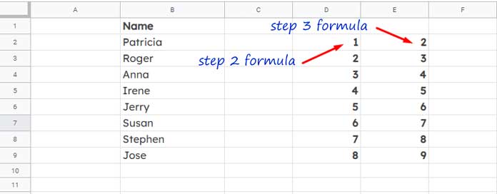
=filter(row(B2:B),B2:B<>"")

Here is the screenshot up to step # 3.

To test the current formulas, delete the name “Anna” in cell B4. The sequential formula in cell D2 will return the numbers 1 to 7. But the row number formula in cell E2 will return the numbers 2 to 9 excluding the number 4.

Step # 4:

Actually this is our final formula. This Vlookup generic formula will help you understand the final formula in cell A1.

vlookup(row numbers 2 to n,{step#3 formula,step#2 formula},2,0)

To understand the above Vlookup generic formula, you must follow the Vlookup syntax which is as follows.

VLOOKUP(search_key, range, index, [is_sorted])

search_key – The search keys in Vlookup are row numbers from 2 to n (infinite).
rage – A two-column range formed by {step#3 formula,step#2 formula}
index – No. 2, means step#2 formula.

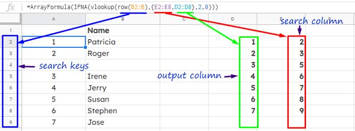
If any of the search keys are found in the formula # 3 output (first column in the rage), the corresponding values from formula # 2, i.e. second column, output will be returned. I have tried to well illustrate that below.

Formula Explanation - Skip Blank Rows in Row Numbering

Currently, as per the illustration above, I have the formula in cell A2. In my final formula I have moved the formula from cell A2 to A1 to place the header “Sr. No.” Scroll up to see the final formula to understand that part.

This way wan we can skip blank rows in sequential numbering in Google Sheets.

Do note that the blank rows are the condition in the above-advanced auto row numbering in Google Sheets.

What about some other conditions instead of blank rows?

Conditional Auto Sequential Numbering in Google Sheets

Here is the formula used in example 2 above (second screenshot from the top) for auto row numbering.

={"Sr. No.";ArrayFormula(ifna(vlookup(row(B2:B),{filter(row(B2:B),(C2:C=false)*(C2:C<>"")),sequence(countif(C2:C,false),1)},2,0)))}

In this formula, the conditions to insert row numbers are the False values in column C. I hope you know that the unchecked checkbox has a value of False.

Formula Explanation – Conditionally Skip Rows in Sequential Numbering (Array Formula)

See how the above formula conditionally skips rows in sequential row numbering in Google Sheets.

Step # 1:

=countif(C2:C9,false)

The above Countif formula (refer my Google Sheets function guide for more info on this function) counts the rows contain False (unchecked checkboxes).

Step # 2:

=sequence(countif(C2:C,false),1)

It goes without saying, right?

Step # 3:

=filter(row(B2:B),(C2:C=false)*(C2:C<>""))

Filters row numbers if the value in C2:C is False and not blank. I have used not blank (C2:C<>"") because Filter treats blank cells as False.

Must Check: How to Use AND, OR with Google Sheets Filter Function.

Here in this screen capture, the Step # 2 formula is in cell E2 and Step # 3 formula is in cell D2.

Step # 4:

This follows the same generic formula (Vlookup) given in the earlier Step # 4. Please follow that.