In this tutorial, we’ll explore two methods to add a specified (n) number of blank rows to SEQUENCE results in Google Sheets. We’ll cover both single-column and grid-based SEQUENCE outputs.

For instance, the following formula will return the numbers 1 to 10 in a column:

=SEQUENCE(10)

To obtain sequential numbers in a grid, i.e., 10 rows by 4 columns, you can use the formula below:

=SEQUENCE(10, 4)

We will use a simple formula to add n blank rows to the SEQUENCE result in a single column.

Regarding the grid output, we will employ a different, slightly more complex formula that will also work in the single-column case.

Adding N Blank Rows to Single-Column SEQUENCE Result

Before entering any formula that returns an array result, ensure sufficient blank cells; otherwise, it will return a #REF! error.

You May Like:- How to Remove #REF! Errors in Google Sheets (Even When IFERROR Fails).

Suppose you want the sequence numbers 1 to 10 with 2 blank rows in between. You can use the following formula for that in Google Sheets:

Formula #1:

=TOCOL(IFNA(HSTACK(SEQUENCE(10),,)))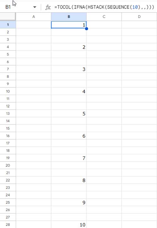

To add 5 blank rows to a single-column SEQUENCE result, use the following formula:

Formula #2:

=TOCOL(IFNA(HSTACK(SEQUENCE(10),,,,,)))

The ‘n’ is determined by the number of commas immediately after the SEQUENCE function, which I’ve highlighted in the formulas above.

Here is the breakdown of Formula #1:

• SEQUENCE(10): returns 10 sequential numbers from 1 to 10.
• HSTACK(…,,): Appends two empty cells.

When you horizontally stack two arrays—one being a sequence with 10 rows and the other containing two empty cells—the HSTACK function returns #N/A errors in the additional rows of the smaller array to align their dimensions.

• IFNA(…): Removes error values with an empty string.
• TOCOL(…): Converts the three-dimensional array (sequence numbers in the first column and two empty columns) into a single column.

The output of TOCOL will be two blank cells inserted between each sequence number.

Adding N Blank Rows to Grid SEQUENCE Results

Unlike our previous example, this may not be a common scenario. But in some cases, you might use the SEQUENCE function to get a 2D array as follows:

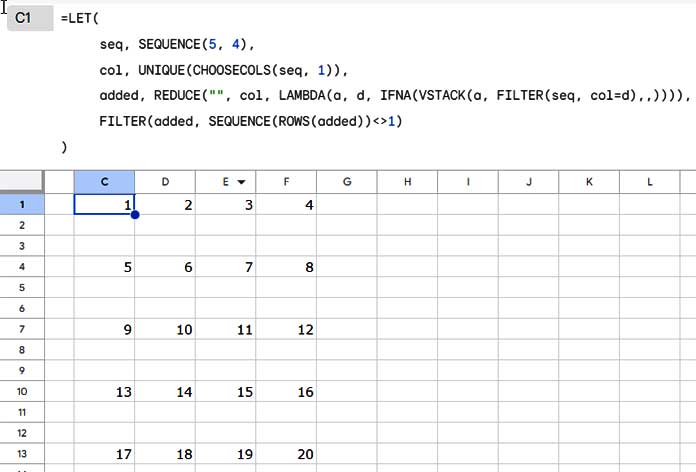
=SEQUENCE(5, 4)

This will return a 5 rows x 4 columns array where the first row will contain the numbers 1 to 4, the second row 5 to 8, the third row 9 to 12, and so forth.

How do we insert a specified number of blank rows within a grid of sequential numbers in Google Sheets?

Here is an example.

Formula #3:

=LET(
     seq, SEQUENCE(5, 4), 
     col, UNIQUE(CHOOSECOLS(seq, 1)), 
     added, REDUCE("", col, LAMBDA(a, d, IFNA(VSTACK(a, FILTER(seq, col=d),,)))), 
     FILTER(added, SEQUENCE(ROWS(added))<>1)
)

The above formula will generate the sequence with 2 blank rows added in between.

Here, the commas in the VSTACK, immediately after the FILTER function, control the number of blank rows inserted.

To add 3 blank rows to a grid SEQUENCE in size 10 rows x 5 columns, replace SEQUENCE(5, 4) with SEQUENCE(10, 5) and VSTACK(a, FILTER(seq, col=d),,) with VSTACK(a, FILTER(seq, col=d),,,).

What’s more! You can even use this formula to insert blank rows between sequential numbers in a single column. Just adjust the SEQUENCE accordingly. For example, instead of the syntax SEQUENCE(rows, columns), use SEQUENCE(rows).

This formula is slightly complex, so understanding it will clarify how the formula adds blank rows in 2D SEQUENCE results in Google Sheets.

Formula Break-Down

We use the LET function to name value expressions, allowing us to use these names in subsequent expressions or the formula itself. This minimizes repetition and enhances overall formula performance.

Syntax:

LET(name1, value_expression1, [name2, …], [value_expression2, …], formula_expression)

Names and Value Expressions:

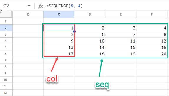
• seq: SEQUENCE(5, 4) creates a 5×4 grid of numbers from 1 to 20.
• col: UNIQUE(CHOOSECOLS(seq, 1)) extracts unique values from the first column of seq.

• added: REDUCE("", col, LAMBDA(a, d, IFNA(VSTACK(a, FILTER(seq, col=d),,)))) the key part of the formula that inserts n (specifically 2 here) blank rows between the sequence numbers.

Here is how the REDUCE works:

REDUCE("", col, LAMBDA(a, d, …): The REDUCE function takes two arguments: an initial value (an empty string in our formula) and an array (col).

The initial value is defined as a, and each value in col, i.e., {1; 5; 9; 13; 7} (please refer to the above image), is defined as d.

The REDUCE function iterates through col, applying a function to each unique value d. d will be the first value in col in the first row, the second value in col in the second row, and so on.

LAMBDA(a, d, …): Defines an anonymous function that processes each value.

IFNA(VSTACK(a, FILTER(seq, col=d),,)): Filters rows from seq where col=d, stacks them below a, and then stacks two empty cells below that. The IFNA handles potential errors due to stacking a one-dimensional array below a 2D array.

The formula extracts each row from the sequence grid and adds blank rows below that using VSTACK. In short, it rearranges the grid of data.

Formula Expression:

Since the initial value in the accumulator is an empty string, there will be a blank row at the top of the result in added.

FILTER(added, SEQUENCE(ROWS(added))<>1)

Removes the initial row from ‘added’ as it’s likely a blank row resulting from the first iteration of REDUCE.

Resources

This tutorial covers the addition of n blank rows to SEQUENCE results (one-dimensional or 2D) in Google Sheets. Here are a couple of tutorials that address a similar topic.

• Skip Blank Rows in Sequential Numbering in Google Sheets
• How to Populate Sequential Dates Excluding Weekends in Google Sheets
• Assign the Same Sequential Numbers to Duplicates in a List in Google Sheets
• Auto-Fill Sequential Dates When Value Entered in Next Column in Google Sheets
• Insert Sequential Numbers Skipping Hidden | Filtered Rows in Google Sheets
• Sequence Numbering in Merged Cells In Google Sheets
• How to Insert Blank Rows Using a Formula in Google Sheets
• How to Automatically Insert a Blank Row below Each Group in Google Sheets
• Insert Blank Rows to Separate Week Starts/Ends in Google Sheets