To auto-fill sequential dates in Google Sheets, you can use either the fill handle or a formula-based approach. This guide will walk you through both methods, including how to auto-fill dates dynamically when values are entered in the next column.
Method 1: Use Fill Handle to Auto-Fill Sequential Dates
The fill handle is the simplest way to auto-fill sequential dates in Google Sheets.
Here’s how it works:
- Enter a date in cell A1, e.g.,
01 Nov 2019. - Enter the next date in A2, e.g.,
02 Nov 2019. - Select both cells (A1:A2), then double-click the fill handle (the small dot or circle at the bottom-right corner of the selection).
Result: Google Sheets will auto-fill sequential dates down the column, continuing until the last row that contains data in the adjacent column.
Note: If you add more values in the next column later, you’ll need to repeat this step manually to extend the date range.
For example, if you later enter values in B15, B16, and B17, you’ll have to select A13 and A14 and double-click the fill handle again to extend the sequence.
Let’s automate that next.
Method 2: Use a Formula to Auto-Fill Sequential Dates
You can auto-fill sequential dates in Google Sheets using an array formula that adjusts based on the number of non-blank rows in the adjacent column.
Example Formula
=SEQUENCE(COUNTA(B1:B), 1, DATE(2019, 11, 1))Steps:
- Format column A as Date (Format > Number > Date).
- Enter the above formula in cell A1.
This formula auto-fills sequential dates in column A, starting from 01 Nov 2019, based on how many values are in column B.
How the Formula Works
- SEQUENCE generates a list of numbers (or dates).
COUNTA(B1:B)counts the number of non-blank rows in column B.DATE(2019, 11, 1)sets the start date.- The result is a column of sequential dates, matching the number of filled cells in column B.
If there are 3 values in B1:B, you’ll get 3 dates in A1:A3.
You can also change the step value to generate alternate dates:
=SEQUENCE(COUNTA(B1:B), 1, DATE(2019, 11, 1), 2)This will return 01 Nov, 03 Nov, 05 Nov, and so on.
Handle Empty Cells in the Adjacent Column
Sometimes, your data in column B might have gaps. There are two ways to handle such cases.
Option 1: Fill Dates Up to the Last Non-Empty Row
If you want to fill sequential dates continuously (including blank rows), use this formula:
=ARRAYFORMULA(SEQUENCE(XMATCH(TRUE, B1:B<>"", 0, -1), 1, DATE(2019, 11, 1)))This version uses XMATCH to find the last non-blank row in column B and fills sequential dates accordingly.

Related: XMATCH First or Last Non-Blank Cell in Google Sheets
Option 2: Fill Dates Only Where Data Exists
If you only want to generate dates where there’s a value in the adjacent cell, skipping blanks, you can use one of the following formulas.
a. Using LAMBDA (for small datasets)
=ARRAYFORMULA(IF(B1:B="",, MAP(B1:B, LAMBDA(cell, DATE(2025, 1, COUNTA(B1:cell))))))COUNTA(B1:cell)counts non-blank cells up to the current row.DATE(2019, 11, …)creates the corresponding date.- Empty cells in column B return blank results in column A.
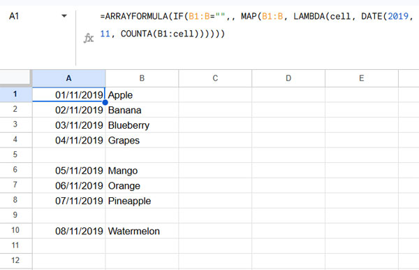
Note: LAMBDAs can be resource-intensive in large datasets.
b. Non-LAMBDA Alternative (for large datasets)
=ARRAYFORMULA(IFERROR(DATE(2019, 11, IF(B1:B="", NA(), COUNTIFS(B1:B, "<>", ROW(B1:B), "<="&ROW(B1:B))))))This formula achieves the same result without LAMBDA, making it more suitable for larger spreadsheets.
How This Works (Explanation)
COUNTIFS(B1:B, "<>", ROW(B1:B), "<="&ROW(B1:B))counts how many non-empty rows appear above (including the current one).IF(B1:B="", NA(), …)ensures blank cells are skipped.
Summary
Using formulas in Google Sheets, you can easily auto-fill sequential dates based on entries in another column. Whether you want to:
- Fill dates continuously until the last filled cell, or
- Generate dates only for filled rows,
Google Sheets offers flexible, formula-based solutions.
Resources
- How to Populate Sequential Dates Excluding Weekends in Google Sheets
- How to Generate Bimonthly Sequential Dates in Google Sheets
- Creating Sequential Dates in Equally Merged Cells in Google Sheets
- Generating a Sequence of Months in Google Sheets
- Adding N Blank Rows to SEQUENCE Results in Google Sheets


