This tutorial elaborates on how to fix most #REF! errors in Google Sheets, as well as how to remove them even when IFERROR fails.

Fixing a formula error is easy if you know the underlying problem. Google Sheets has an error tooltip approach to help users identify problems.

Sometimes, you know the reason for the error and want to forcefully mask the error for the time being. In that case, you may use the IFERROR function.

It can help you replace the #REF! error value with a custom value or a blank cell. But it fails in some cases. We will see two such scenarios and how to mask the error in those cases using another formula or conditional formatting.

In my tutorial titled “Different Error Types in Google Sheets and How to Correct Them“, I already touched on this, but I focused on all 8 error types. Also, the IFERROR fail case is not part of that tutorial.

This is a detailed tutorial on how to fix or remove #REF! errors in Google Sheets.

VLOOKUP Out-of-Bounds Range Error

The VLOOKUP out-of-bounds range error happens when you use the wrong index number. Assume the range contains 5 columns. You can specify the numbers 1-5 as the index number in VLOOKUP.

Syntax of the VLOOKUP Function:

VLOOKUP(search_key, range, index, [is_sorted])

In the following example, my formula returns a #REF! error:

=VLOOKUP(A1,A4:E,6,0)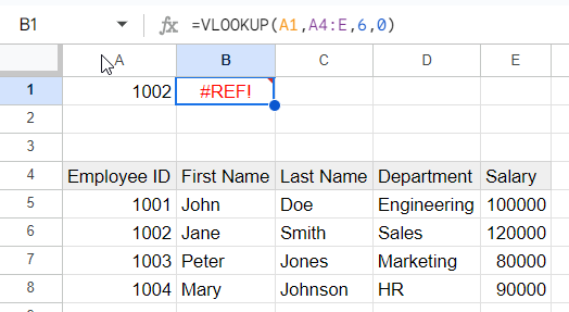

My purpose was to search for an employee ID and return their salary. The salary is in the 5th column, but I specified 6, so the formula returns the out-of-bounds range #REF! error.

Fix Out-of-Bounds Range #REF! Errors in Google Sheets

To troubleshoot the out-of-bounds range #REF! error, correct the index number in the formula as follows:

=VLOOKUP(A1,A4:E,5,0)

This is also applicable when using the HLOOKUP function in Google Sheets, but the row index is the cause of the error in that case.

Remove Out-of-Bounds Range #REF! Errors in Google Sheets

You can remove this #REF! error in VLOOKUP in Google Sheets with the IFERROR function:

=IFERROR(VLOOKUP(A1,A4:E,6,0),"")

This will return an empty string if the VLOOKUP formula returns an error.

Replace "" with a custom text if you want to return something else instead of an empty string.

Tip: I highly suggest using IFNA with functions that can return #N/A errors, such as VLOOKUP, HLOOKUP, XLOOKUP, MATCH, XMATCH, and FILTER.

Circular Dependency Detected Errors

This usually happens when a formula refers to the cell that it is entered into. If you did this purposefully, you need to turn on iterative calculation by going to File > Settings > Calculation and selecting Iterative calculation. Otherwise, it would be best if you corrected the formula.

Here is an example of a circular dependency detected error in Google Sheets:

=SUM(C2:C5)

This formula is in cell C5 and refers to the range C2:C5, which includes the cell itself. This creates a circular dependency.

Fix Circular Dependency Detected #REF! Errors in Google Sheets

To correct the error, as per my example, replace the range in the formula with C2:C4. This will exclude the cell itself from the range and eliminate the circular dependency.

=SUM(C2:C4)

Remove Circular Dependency Detected #REF! Errors in Google Sheets

You cannot replace this error with an empty string using the IFERROR function in Google Sheets. This is one case where IFERROR fails.

=IFERROR(SUM(C2:C5),"") // It will return a #REF! error

To remove (mask) this error, you need to use two conditional format rules:

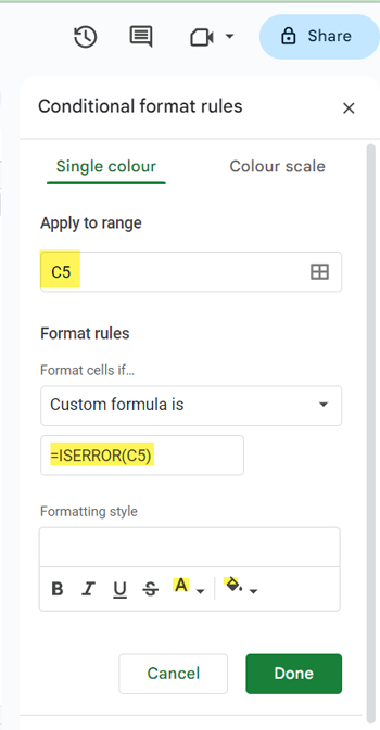
Mask the error:

• Click Format > Conditional formatting.
• In the Custom formula is field, enter the following formula:

=ISERROR(C5)

• Under Formatting style select Text color > White and Fill color > None
• Click Done.

Unmask the error if the cell doesn’t have an error:

• Click Format > Conditional formatting> Add another rule.
• In the Custom formula is field, enter the following formula:

=NOT(ISERROR(C5))

• Under Formatting style select Text color > Black and Fill color > None
• Click Done.

This will hide the error message and display the value of cell C5 if it doesn’t contain an error.

Deleting a Row or Column and #REF! Errors

This usually occurs when you delete a row or column that has been referenced in a formula. You may not see any tooltip associated with the formula, so check the formula itself to find the reason.

In the following XLOOKUP formula, the #REF! error replaces the lookup range because I deleted the lookup range:

=XLOOKUP("Apple",#REF!,A:A)

This was the working formula:

=XLOOKUP("Apple",A:A,B:B)

How to Fix It

There is no specific fix to this problem. You need to edit the formula and replace #REF! with the proper cell references. Also, you may need to modify other cell references in the formula which may have been adjusted due to deleting rows or columns.

How to Remove It

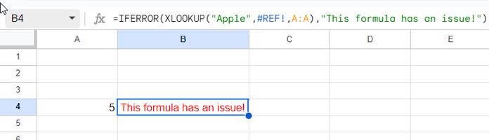
We can remove the #REF! error caused by removing a row or column in Google Sheets using IFERROR as follows:

=IFERROR(XLOOKUP("Apple",#REF!,A:A),"This formula has an issue!")

This will return a custom text if the XLOOKUP formula returns an error.

REF! Error Caused by Mismatched Row Sizes in Concatenated Arrays

When you combine two arrays using curly braces, the number of rows in both arrays must match. Otherwise, the formula will return a #REF! error.

This error usually occurs when you combine two QUERY results or other formula results horizontally in Google Sheets.

Here is a basic example in which I am combining two unequal-sized arrays horizontally:

={B2:B6,C2:C5}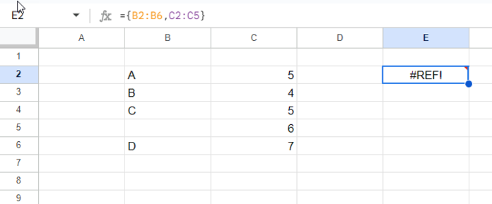

Fix #REF! Errors Caused by Curly Braces with HSTACK

We can fix this error by replacing the curly braces with the HSTACK function in Google Sheets:

=HSTACK(B2:B6,C2:C5)

Related: ARRAY_ROW Function #REF! Error and Solution in Google Sheets

How to Remove It

Can we remove such #REF! errors using the IFERROR function? Yes, we can:

=IFERROR({B2:B6,C2:C5},"This formula has an issue!")

Array Result Was Not Expanded Error

This happens when a formula that returns values in more than one cell can’t fill the cells due to existing values.

How to Fix It

To fix this error, you can:

• Hover your mouse pointer over the formula to find the cell that causes the problem and remove the value in that cell. You may need to do this multiple times.
• Use the ARRAY_CONSTRAIN function to constrain the size of the output.

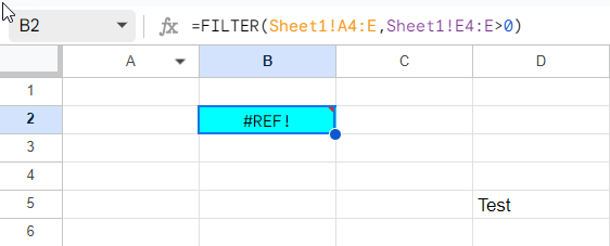
For example, the following FILTER formula in cell B2 returns the #REF! error because it can’t expand down:

=FILTER(Sheet1!A4:E,Sheet1!E4:E>0)

This formula returns a 5 x 5 matrix, but the value in cell D5 breaks it.

If you want to keep the value in cell D5, you need to move the formula to a different range or limit the number of rows or columns in the result.

You can use the ARRAY_CONSTRAIN function to limit the result to 3 rows as a value in the fourth row causes the issue:

=ARRAY_CONSTRAIN(FILTER(Sheet1!A4:E,Sheet1!E4:E>0),3,5)

Remove Array Result Was Not Expanded #REF! Errors in Google Sheets

In this case, we can’t use the IFERROR function to remove the error. You need to use Conditional Formatting or a workaround solution.

The “circular dependency” and the “array result was not expanded”, resulting in the two #REF! errors where the IFERROR function fails miserably.

In the case of circular dependency, we have used two highlight rules to mask the error. You can use the same two rules here.

In addition, you can use a helper cell to remove the “array result that was not expanded” error in Google Sheets.

Steps:

In a helper cell that must not fall in the formula expansion range (such as a cell to the left or top of the formula-applied cell), create a drop-down that contains two values: Yes and No. For example, if your formula is in cell B2, you could create the drop-down in cell A2.

To create the drop-down:

• Go to cell A2 and click Insert > Drop-down.
• Replace Option 1 with Yes and Option 2 with No.
• Click Done.

To remove a #REF! error caused by an array result that was not expanded, you need to replace your formula with the following:

=IF(A2="No",,formula_here)

Replace formula_here with your original formula.

For example, if your original formula is:

=FILTER(Sheet1!A4:E,Sheet1!E4:E>0)

Your new formula would be:

=IF(A2="No",,FILTER(Sheet1!A4:E,Sheet1!E4:E>0))

Once you have replaced your formula, select No in cell A2.

The formula will return blank.

When you clear the area for the formula to expand, choose Yes in cell A2.

This will prevent the #REF! error from appearing.

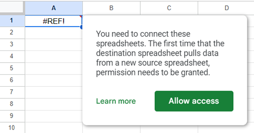
Allow Access IMPORTRANGE Error

When you use the IMPORTRANGE function to import data from one Sheet to another, the formula will return a #REF! error if you have not authorized access to the source Sheet.

Fix #REF! Errors Caused by IMPORTRANGE

If you own the source Sheet:

1. Hover your mouse over the error and click the Allow access button.

If you do not own the source Sheet:

1. Copy the spreadsheet URL from the formula.
2. Open a new tab in your browser and paste the URL.
3. Click the Request Access button and wait for the spreadsheet owner to grant you access.

How to Remove It

To remove the IMPORTRANGE #REF! error, wrap the formula with the IFERROR function.

Conclusion

We have seen different types of #REF! errors in Google Sheets and how to fix and remove them. It is more important to fix the errors than to remove them.

I suggest using the IFERROR function to remove trailing error values in blank rows when using array formulas.