Let’s learn about different error types in Google Sheets and how to correct them.

When the formula in a cell has an error, Google Sheets returns an error value.

To make things easier for users, Google Sheets returns different error values for different error types. All of these error values start with the # number sign.

To correct a formula error in Google Sheets, you must understand the error values.

Different Error Types in Google Sheets

All of the following formula error values have a number associated with them:

1. #NULL! (error type 1)
2. #DIV/0! (error type 2)
3. #VALUE! (error type 3)
4. #REF! (error type 4)
5. #NAME? (error type 5)
6. #NUM! (error type 6)
7. #N/A (error type 7)
8. All other error types (error type 8)

These are the 8 different error types in Google Sheets. If any of the cells contain error values, you can use the ERROR.TYPE function to test it and get the error numbers in another cell.

The ERROR.TYPE function can identify all of the above 8 types of errors in Google Sheets and return the numbers from 1 to 8 accordingly.

How to Use the Error.Type Function in Google Sheets

Syntax of the Google Sheets ERROR.TYPE function:

ERROR.TYPE(REFERENCE)

Arguments:

• reference: The cell or expression to find the error number for.

Usage:

Suppose cell A1 has an error value #DIV/0!. The following formula would return 2:

=ERROR.TYPE(A1)

Alternatively, you can use the formula in cell A1 itself with the ERROR.TYPE function:

=ERROR.TYPE(5/0)

How to Use Error Numbers in Google Sheets

Error numbers in Google Sheets can be used to identify and troubleshoot formula errors. They can also be used to create custom error messages and to control the behavior of formulas when errors occur.

Example:

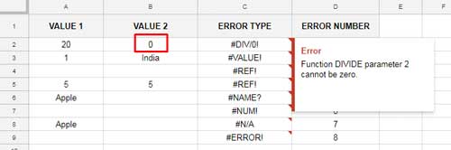
Suppose cell A1 contains the value 20 and cell B1 contains the value 0. The following formula will return an error:

=A1/B1

The result of the formula will be the error code #DIV/0!. This error code indicates that the formula is trying to divide by zero, which is not allowed in Google Sheets.

If you hover your mouse over the cell containing the formula, you will see a tooltip that says “Function DIVIDE parameter 2 cannot be zero”. This tooltip provides more information about the error and how to fix it.

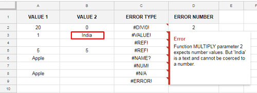
See one more example. Here Value in A1 is 20, and B1 is a text string.

=A1/B1

The result of the formula will be #VALUE! because it is trying to divide a number by a text string.

Here we can use Google Sheets ERROR.TYPE function as below in an IF logical test.

=IFERROR(
   IF(ERROR.TYPE(A1/B1)=2,
      "Value Can't Be Zero",
      IF(ERROR.TYPE(A1/B1)=3,
         "Value Can't Be Text")
   ),A1/B1
)

This formula would return “Value Can’t Be Zero” if the error type is #DIV/0!, “Value Can’t Be Text” if the error type is #VALUE!, else the final part A1/B1.

Do you know why I’ve used the IFERROR function in this formula?

The ERROR.TYPE function itself returns an #N/A error if there is no error in the calculation.

So if the error value is #N/A, we can decide that there is no error in our formula. With the help of IFERROR, we can execute the A1/B1 calculation.

You have already learned about different error types in Google Sheets and the use of Google Sheets ERROR.TYPE function.

Now is the time to learn in detail about all error types and how to correct them in your Spreadsheet.

You May Also Like: Difference Between ISERR and ISNA Functions in Google Sheets

Understand Error Values in Google Sheets

1. #NULL!

I’ve never seen the #NULL! error in Google Sheets, although it does exist in Excel.

In Google Sheets, the error number associated with it is 1. This may be for cross-platform compatibility.

2. #DIV/0! Error in Google Sheets and How to Correct It

It’s easy to correct the #DIV/0! error in Google Sheets. See the example below.

The error occurs because the value in cell B2 is 0. The value in cell B2 should not be 0 or blank.

I’ve applied the formula in cell C1. Check the error notification in that cell.

3. #VALUE! Error in Google Sheets and How to Correct It

The #VALUE! error is one of the most commonly occurring errors in Google Sheets. It occurs when you apply mathematical operations to one or more cells that contain text strings.

In the example below, the multiply function encounters an error because the value in cell B3 is text. However, even if the values are numbers, you may still see this error if the numbers in the reference cells are formatted as text. You can check the formatting by going to Format > Number.

You May Like:- How to Sum, Multiply, Subtract, and Divide Numbers in Google Sheets.

4. #REF! Error in Google Sheets and How to Correct It

There are five main reasons for the #REF! error in Google Sheets:

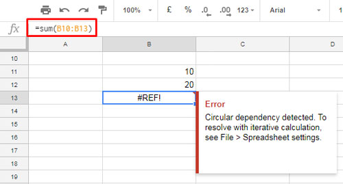
1. Circular dependency: This occurs when a formula refers to itself, either directly or indirectly. For example, the formula in cell B3 in my example (see screenshot below) would create a circular dependency, because it refers to cell B13, which in turn refers to cell B3.
2. Deleted reference cell: If you delete a cell, row, column, or sheet that is referenced in a formula, you will get the #REF! error. It can be difficult to correct such formulas, but it is possible.
3. Array formula expansion failure: This can occur when an array result is not able to be expanded because it would overwrite data.
4. Unequal-sized arrays: If you combine two arrays of different sizes in a formula, you will get the #REF! error. (See the ARRAY_ROW undocumented function for more information.)
5. Out-of-bounds range: A common issue in lookup functions occurs when the result range is outside the given range.

Related: How to Remove #REF! Errors in Google Sheets (Even When IFERROR Fails)

5. #NAME? Error in Google Sheets and How to Correct It

The following logical test is a good example of why Google Sheets returns the #NAME? error:

=IF(A6*Apple,"Yes","No")

If you have a cell named “Apple” and it contains any number or is left blank, the formula will work correctly.

6. #NUM! Error in Google Sheets and How to Correct It

The #NUM! error is rare to see in Google Sheets, but it can occur when a formula contains an invalid argument. For example, the following RATE formula would return the #NUM! error:

=RATE(75, -1500, -10000, 200000)

To correct the formula you should check the arguments in the function.

7. #N/A Error in Google Sheets and How to Correct It

The #N/A error is the most common error in Google Sheets. It means that the value is not available or does not match the expected value.

Example:

Cell value in A8: “Apple”

The following formula would return the #N/A error:

=IFS(A8="Orange",500)

This is because the value in cell A8 is “Apple”, not “Orange”.

The following formula would return Boolean FALSE:

=IF(A8="Orange",500)

This is because the condition in the IF statement is not met.

Related: How to Use the Google Sheets IFNA Function

Other error types, usually associated with a typo, are displayed as #ERROR!

Example:

Formula:

=SUM(A9 b9)

Result: #ERROR!

This is because there is a space between the cell references A9 and b9. The correct syntax is =SUM(A9,B9).

Conclusion

This tutorial has shown you the different error types in Google Sheets and how to correct them. I hope this is helpful!