What causes the ARRAY_ROW function #REF error in Google Sheets formulas? Is there any such function hidden somewhere in my code?
As far as I know, the ARRAY_ROW is an undocumented function in Google Sheets.
The purpose of this function is to combine equal-sized arrays/ranges, in terms of number of rows, horizontally.
We usually use curly brackets to combine two or more equal-sized ranges horizontally. We can use the ARRAY_ROW function instead.
Both will return a #REF error in case of mismatched ranges. If you hover your mouse over the error, you will see function ARRAY_ROW parameter ‘n’ has a mismatched row size.
ARRAY_ROW Function Syntax and Arguments
Before explaining how to remove the ARRAY_ROW function #REF error, let’s try to understand this simple function.
I couldn’t find any official documentation of the ARRAY_ROW function in Google Sheets. I think we can best write its syntax as follows.
Syntax: ARRAY_ROW(range1, [range2, …])
range1: The first range to combine horizontally.
range2, ...: Additional ranges to combine to range1. The number of rows in the additional ranges should match with range1.
Example
In the following example, see how to use the ARRAY_ROW function and curly brackets to append/combine ranges horizontally.
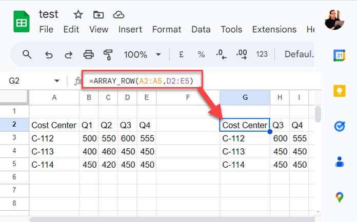
I have cost centers (project codes) in A2:A5 and the total labor strengths in Q1, Q2, Q3, and Q4 in corresponding column ranges, i.e., B2:E5.
How do I copy the cost center and Q3 and Q4 data to a separate range?
We can use the following formula.
=ARRAY_ROW(A2:A5,D2:E5)Alternative Formula: ={A2:A5, D2:E5}
Now time to see the cause of the ARRAY_ROW function #REF error and how to solve it.
ARRAY_ROW Function #REF Error and How to Solve It?
Usually, the said error happens when we use curly brackets to append two or more ranges.
I’m sure most Google Sheets users are not using the ARRAY_ROW function.
For one reason, it’s not a documented function. And the other is there is the much simpler curly braces alternative. We have already seen one example above.
There are two reasons for the ARRAY_ROW function #REF error in Google Sheets. Both reasons are most likely associated with curly braces usage.
- The user may want to combine two ranges or formula results vertically (one below the other). He accidentally placed them side by side (used a comma instead of a semicolon within the curly brackets). So there are chances of mismatching rows in the two ranges.
- When a user intentionally combines two formula results horizontally, which have mismatching row sizes. For example, say two IMPORTRANGE formulas side by side from two sheets.
I’ll show you the error first (the basic one), then come to the solution.
={A2:A10,D2:E5}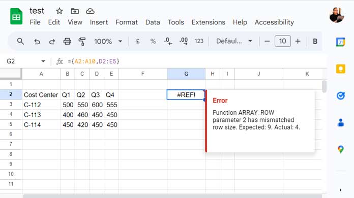
Solution
The solution to the ARRAY_ROW function #REF error depends on whether you really want to append the arrays horizontally.
If you want to append two or more ranges vertically, forget about the curly brackets approach. Use the VSTACK function.
If you want to place two or more ranges side by side, use the HSTACK function. It won’t cause the above #REF error.
In the above example, we can use =HSTACK(A2:A10, D2:E5) instead of the above curly bracket formula. So you won’t see the error.
The formula will place the ranges side by side.
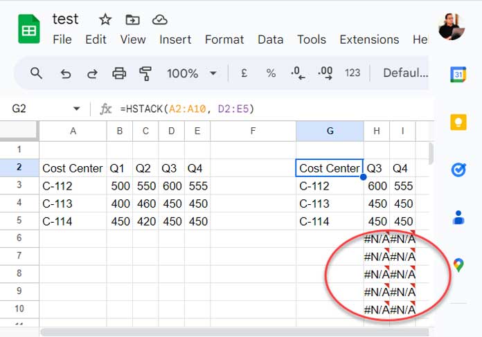
But I suggest wrapping it with IFNA like =IFNA(HSTACK(A2:A10, D2:E5)). There is an obvious reason for it.
HSTACK will add ‘new’ rows below the lesser-sized range, and they contain #NA error values. We can clean it using the IFNA or IFERROR functions.
So to solve the function ARRAY_ROW parameter mismatch row error, use the HSTACK or VSTACK functions in Google Sheets.


