The HSTACK function in Google Sheets is used to append ranges horizontally. While we can use curly braces for this purpose, they cannot fully replace the HSTACK function.
Do you know why?
Curly braces require that all the ranges being appended have the same number of rows.
However, with the HSTACK function, you can use arrays of any size. It does not require the number of rows or columns in the appended ranges to match.
I find the VSTACK function (vertical stacking) more practical than its sibling’s HSTACK (horizontal stacking).
Syntax of the HSTACK Function
Syntax: HSTACK(range1, [range2, …])
- range1: The first array or range to append.
- range2, …: Additional arrays or ranges (optional) to append to the first range.
Example
I have three tables and want to append them horizontally into a single array.
The table ranges are A3:D4, A6:C8, and A9:D10.
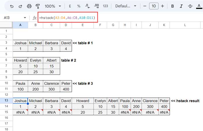
The HSTACK formula in cell A13 returns the single appended array in A13:K15.
=HSTACK(A3:D4, A6:C8, A9:D10)Why are there some #N/A values in the result?
As you can see, the number of rows and columns in each table is different.
But the HSTACK function has no issue appending them horizontally.
The output of the HSTACK formula will have rows equal to the maximum number of rows from the appended ranges
In this process, it adds #N/A values in some cells to fill the gaps where rows are missing.
To remove these #N/A values, wrap the formula with an IFNA function.
=IFNA(HSTACK(A3:D4, A6:C8, A9:D10))HSTACK with SUMIF Function in Google Sheets (Real-Life Example)
Now that we’ve learned how the HSTACK function works in Google Sheets, let’s see a real-life example of using it with the SUMIF function to generate a summary table.
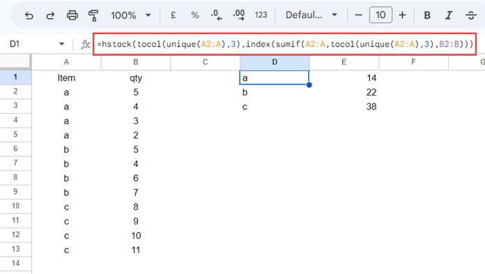
Assume we have a product list in column A and their quantities in column B.
How do we create a summary from this data?
Of course, the following QUERY formula will do that:
=QUERY(A:B, "SELECT A, SUM(B) WHERE A IS NOT NULL GROUP BY A", 1)Alternatively, we can use UNIQUE and SUMIF functions combined with HSTACK, as shown below:
=HSTACK(
   TOCOL(UNIQUE(A2:A), 3),
   INDEX(SUMIF(A2:A, TOCOL(UNIQUE(A2:A), 3), B2:B))
)
Let’s break this formula down:
- range1:
TOCOL(UNIQUE(A2:A), 3)
This returns the unique items from column A without blanks. - range2:
INDEX(SUMIF(A2:A, TOCOL(UNIQUE(A2:A), 3), B2:B))
This returns the sum of quantities for each unique product.
The HSTACK function appends these two ranges horizontally, giving us a summary of products and their total quantities.
I hope the above examples help you understand how to use the HSTACK function in Google Sheets effectively.


