The UNIQUE function in Google Sheets is designed to return either unique or distinct values from a list or table range. It can operate either row-wise or column-wise based on your preference.
The terms “unique values” and “distinct values” are often used interchangeably, but in this context, there is a difference in their meaning.
Unique: For instance, in a list of names, the UNIQUE function can eliminate multiple occurrences of names, if any, and provide a list of unique names.
Distinct: In the same list of names, the function will only return names that have no duplicates or multiple occurrences.
It’s worth noting that in some online tutorials, you may not come across this distinction. Initially, the function didn’t have a distinct feature; it was added later on. Another noteworthy change in the function over the years is its improved capability to handle both vertical and horizontal datasets.
Syntax and Arguments of the UNIQUE Function in Google Sheets
Syntax of the UNIQUE Function in Google Sheets:
UNIQUE(range, [by_column], [exactly_once])Arguments:
range: The range or array from which to return unique rows or columns.by_column: Use either TRUE or FALSE boolean values. TRUE means unique/distinct by column, and FALSE means unique/distinct by row.exactly_once: Use either TRUE or FALSE boolean values. TRUE will return all distinct rows/columns that occur exactly once. FALSE will remove multiple occurrences and return the rest of the rows/columns.
The last two arguments are optional and set to FALSE by default.
Examples of the UNIQUE Function in Google Sheets
In this basic example section, let’s explore the understanding of all the arguments in the UNIQUE function.
This will help clarify the distinction between unique and distinct values in the UNIQUE function perspective, as well as illustrate how the function operates with data in both rows and columns. We will begin by examining data arranged in rows.
Return Unique and Distinct Values in a Row-Wise List
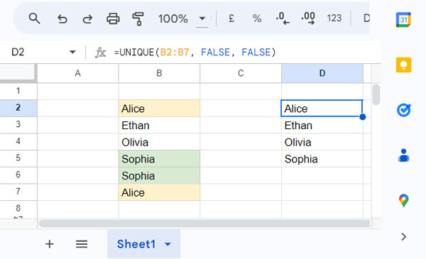
In the following examples, I have a list of names in the range B2:B7, and they are {Alice, Ethan, Olivia, Sophia, Sophia, Alice}.
As you can see, “Alice” and “Sophia” occur twice. To obtain the unique names from this vertical data range, you can use the following formula:
=UNIQUE(B2:B7, FALSE, FALSE)Where:
range: B2:B7by_column: FALSEexactly_once: FALSE
It will return the names {Alice, Ethan, Olivia, Sophia}.
Since the last two arguments are optional and their default values are FALSE, you can omit using them in the formula:
=UNIQUE(B2:B7)This is the most common use case of the UNIQUE function in Google Sheets.
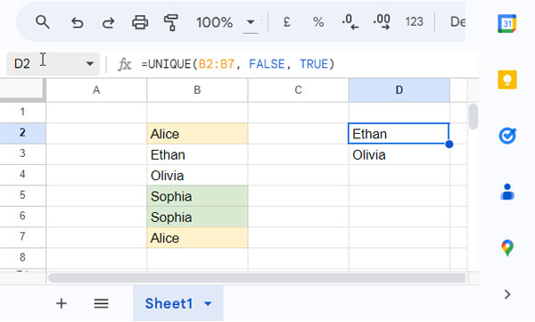
In the list, the distinct names are “Ethan” and “Olivia.” To obtain those names, use the following UNIQUE formula:
=UNIQUE(B2:B7, FALSE, TRUE)Where:
range: B2:B7by_column: FALSEexactly_once: TRUE
Return Unique and Distinct Values in a Column-Wise List
If the above list of names is in the range B2:G2, arranged in columns, you need to replace the FALSE in the second argument, which is by_column, with TRUE in both unique and distinct formulas.
Here are examples:
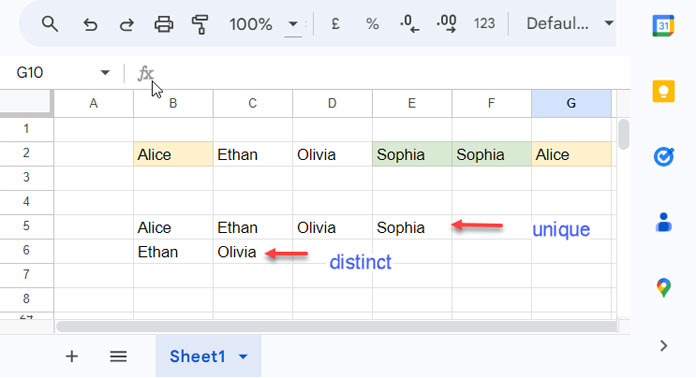
The formula in cell B5 returns unique names in the horizontal data range.
=UNIQUE(B2:G2, TRUE, FALSE)Where:
range: B2:G2by_column: TRUEexactly_once: FALSE
The following formula in cell B6 returns distinct names:
=UNIQUE(B2:G2, TRUE, TRUE) // returns distinct namesWhere:
range: B2:G2by_column: TRUEexactly_once: TRUE
In the above examples, we have used the UNIQUE function either in a single column or a single row. What about a table range?
Utilizing the UNIQUE Function in a Table in Google Sheets
Here, I have a table with three columns, and the data are arranged in rows in the range A1:C5.
The formula in cell F1 is:
=UNIQUE(A1:C5)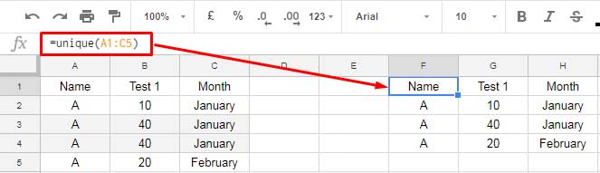
When you use a multi-column table with data arranged in rows, the UNIQUE function takes into account the entire row for evaluating duplicates.
In that sense, A3:C3 and A4:C4 are duplicates, so the function removes one of them.
Note: To get the distinct rows from this range, you can use the following formula: =UNIQUE(A1:C5, FALSE, TRUE)
This can be a drawback in some cases. See the below example to understand it.
Exploring an Alternative
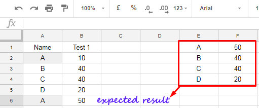
In this example, there are two columns in the provided source range A2:B, the first column contains participants’ names, and the second column contains their test scores.
If a participant has appeared for multiple tests and his scores are the same, the UNIQUE function can remove the duplicate row.
But if his scores are different, it can’t as the function evaluates the entire row for finding duplicates, not any particular column.
We can use the SORTN function instead of the UNIQUE function to solve this problem. Here is a sneak peek.
=SORTN(A2:B, 9^9, 2, 1, 1) // returns the first occurrences of namesNote: You can sort the data by names in ascending order and scores in descending order before applying SORTN to get the rows with the highest scores. Example: =SORTN(SORT(A2:B, 1, TRUE, 2, FALSE), 9^9, 2, 1, 1)
Syntax:
SORTN(range, [n], [display_ties_mode], [sort_column], [is_ascending], [sort_column2, …], [is_ascending2, …])
Where:
range: A2:Bn: 9^9 (use this arbitrarily large number to return all rows after processing)display_ties_mode: 2 (to remove duplicate rows)sort_column: 1 (the column that contains duplicates)is_ascending: 1 (A-Z order)
In this formula, you can specify any individual column containing the duplicates.
The number 1, which is the second from the last in the above formula, indicates the column that contains the duplicates.
To learn more about this, please check out: How to Apply Unique in Selected Columns in Google Sheets
How to Remove Blank Cells in the UNIQUE Function Result in Google Sheets
We often employ the UNIQUE function in row-wise data in Google Sheets. Let’s explore how to eliminate blank cells from the UNIQUE result.
The UNIQUE function includes blank cells in its results. If the range contains one or more blank cells, the formula will return a single blank cell.
If the range is B2:B, you can use the TOCOL function with the UNIQUE function to remove the blank cell.
=TOCOL(UNIQUE(B2:B), 1)This step is crucial because we typically use the UNIQUE result as criteria to aggregate data, and the presence of a blank cell may cause issues.
Note: If you use the UNIQUE function in a multi-column range and want to remove blank rows, please refer to this tutorial: Filter Out If the Entire Row Is Blank in Google Sheets.
Conclusion
The UNIQUE function is case-sensitive in Google Sheets but case-insensitive in Excel. Please keep this distinction in mind if you use both applications.
Case sensitivity is a complex topic when it comes to the UNIQUE function. For a more in-depth exploration, refer to our separate tutorial here: Case-Insensitive Unique in Google Sheets.
In addition to TOCOL, as explained earlier, you can leverage functions like SORT, FLATTEN, QUERY, etc., in combination with the UNIQUE function in Google Sheets.
You can use the SORT function to arrange the unique or distinct results returned by the formula in ascending or descending order.
Syntax: SORT(UNIQUE(range))
To handle unique or distinct scattered values in cells, you can utilize the FLATTEN function within the UNIQUE function using the following syntax:
=UNIQUE(FLATTEN(range))That’s all. Thanks for staying with us. Enjoy!


Hi Sir,
Here I am sharing my Google Sheet link.
I have customer balance confirmation data.
I need to show the customer’s latest balance confirmation (YES ) status in the last three months, all in one place.
URL removed – Admin
Please, guide me on how I can get this through a Google spreadsheet Query.
Hi, B4ALLB4U,
You require a basic Query formula which I have entered in Sheet2!B2.