Google Sheets offers a highly versatile function, SORTN, that enables you to achieve what the UNIQUE function cannot: applying UNIQUE by specific columns. This means you can evaluate uniqueness for selected columns in a dataset instead of considering the entire row.
For instance, in a two-column dataset, you can apply UNIQUE by the first column (field) while retaining data in the second column. This level of flexibility makes SORTN an invaluable tool for advanced data manipulation.
When you use the UNIQUE function on a two-column dataset, it evaluates both columns together. This may not always yield the desired results. Using SORTN, however, you can customize the evaluation to focus on specific columns.
In this tutorial, I’ll show you step-by-step how to apply UNIQUE by specific columns using the SORTN function.
Why Use SORTN Instead of UNIQUE?
The UNIQUE function works well for simple datasets but has its limitations. It evaluates entire rows or columns, which makes it unsuitable when you need to focus on specific columns.
SORTN, on the other hand, provides greater flexibility. It allows you to apply UNIQUE by specific columns while also keeping the data sorted. Think of it as a “Group By” feature, but without aggregation.
Another key difference to note is that UNIQUE is case-sensitive, while SORTN is not. This distinction can be critical depending on your data needs.
Applying UNIQUE to One Column Using the UNIQUE Function
Let’s start with a simple dataset of fruit names in one column. Some fruit names appear multiple times.

Using the formula:
=UNIQUE(A2:A10)the UNIQUE function removes duplicates, leaving only distinct values.
Applying UNIQUE to One Column Using SORTN
With the SORTN function, you can achieve the same result as above but with additional features. Here’s the formula:
=SORTN(A2:A10, 9^9, 2, 1, TRUE)This formula also removes duplicates, but the result is sorted by default.

Key Elements in the SORTN Formula:
9^9: A constant value required for Tie Mode 2.2(Tie Mode 2): Activates advanced UNIQUE behavior.1(Sort Column): Specifies the column to evaluate for uniqueness. Adjust this for specific columns. Note that you can use either the column index number or a range reference, such asA2:A10.TRUE: Sorts in ascending order. UseFALSEfor descending order.
Applying UNIQUE by Specific Columns in Two-Column Datasets
Using UNIQUE
In a two-column dataset (e.g., fruit names in column A and prices in column B), the UNIQUE function considers both columns together. For example:
=UNIQUE(A2:B11)If the same fruit appears with different prices, each instance is treated as unique.

Using SORTN
With SORTN, you can customize the evaluation:
UNIQUE by Both Columns:
=SORTN(A2:B11, 9^9, 2, 1, TRUE, 2, TRUE)This formula evaluates both columns for uniqueness, similar to the UNIQUE function. Note that the result will be sorted.
In this formula, two sort columns are specified. The elements 1, TRUE, 2, TRUE after the tie-mode number define the columns to evaluate for uniqueness. As a result, the formula ensures both columns are considered when determining unique rows.
UNIQUE by Specific Column (First Column Only):
=SORTN(A2:A10, 9^9, 2, 1, TRUE)This evaluates only the first column while retaining data from the second column.

Using SORTN to apply UNIQUE by specific fields is especially useful when working with grouped data or when you need to retain contextual information from other columns.
Applying UNIQUE by Specific Columns in Three-Column Datasets
For datasets with three columns, SORTN allows you to evaluate uniqueness based on any combination of columns.
For example, to apply UNIQUE by fields 1 and 3, use:
=SORTN(A2:C11, 9^9, 2, 1, TRUE, 3, TRUE)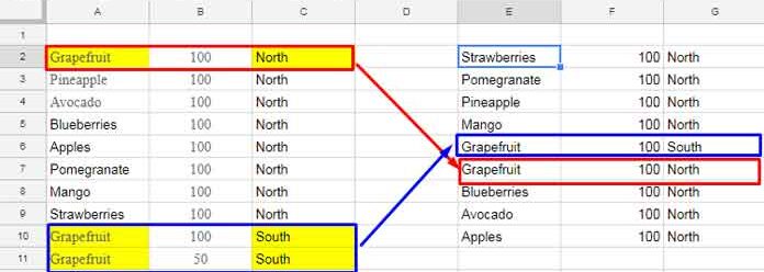
Conclusion
Learning how to apply UNIQUE by specific columns in Google Sheets can be a game-changer for data manipulation. Functions like SORTN provide unparalleled flexibility, surpassing the limitations of the UNIQUE function.
By mastering SORTN and understanding Tie Mode 2, you’ll unlock advanced techniques for working with complex datasets. However, keep in mind that UNIQUE is case-sensitive, whereas SORTN is not.
Explore this powerful function to elevate your Google Sheets skills to the next level!
Resources
- Case Insensitive Unique in Google Sheets
- Count Unique in Google Sheets QUERY
- How to Return Unique Rows in Google Sheets QUERY
- How to Unique Rows Ignoring Timestamp Column in Google Sheets
- How to Use COUNTIF with UNIQUE in Google Sheets
- How to Use UNIQUE and SUM Together in Google Sheets
- Highlighting Distinct and Unique Values in Google Sheets
- UNIQUE Function in Visible Rows in Google Sheets


You really save the day man!! 🙂
I used your example to construct a duplicates filter formula that works awesome 🙂
Thank you very much!!!