Instead of using the FLATTEN function, we can now use the TOCOL function to transform an array or range of cells into a single column in Google Sheets.
You can use TOCOL(range) or FLATTEN(range) to convert an array into a column. Both formulas will produce the same result and process the data row by row.
However, the TOCOL function offers more flexibility with additional arguments that allow users to remove blank and error values from the range during the conversion.
Additionally, TOCOL can scan the array by column, which is something FLATTEN cannot do directly. In FLATTEN, if you want to scan by column, you need to specify the ranges (one-dimensional) separately as range1, range2, ….
We typically use FLATTEN to unpivot a table. If you use TOCOL for the same purpose, you can control the order of the labels in the unpivoted range.
We will cover that in a later section of this guide.
Syntax and Arguments
Syntax: TOCOL(array_or_range, [ignore], [scan_by_column])
- array_or_range: The array or cell range to return as a column.
- ignore: The default is 0 (no values ignored). You can specify:
- 0 (no values)
- 1 (blanks)
- 2 (errors)
- 3 (blanks and errors).
- scan_by_column: Determines whether the array is scanned by column (TRUE) or row (FALSE). The default is FALSE.
TOCOL Function Examples in Google Sheets
The following TOCOL formula in cell B9 transforms the cell range B2:D5 into a single column, scanning the values by column:
=TOCOL(B2:D5, 0, TRUE)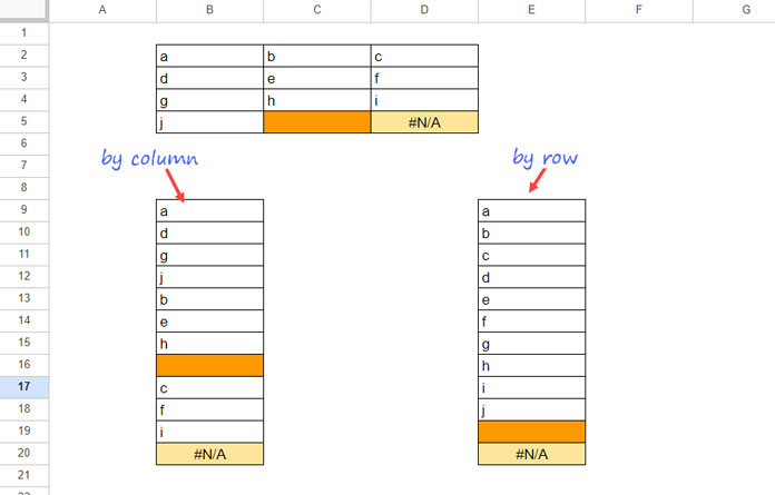
The formula in E9 does the same but scans the values by row.
=TOCOL(B2:D5, 0, FALSE)In both results, you will see a blank cell and an error value. You can remove either one or both by replacing 0 with 1, 2, or 3. For example, to remove both, you can use the following formula:
=TOCOL(B2:D5, 3, FALSE)TOCOL Function for Unpivoting a Table in Google Sheets
You may already be familiar with using the FLATTEN function to unpivot a dataset in Google Sheets. TOCOL can also handle this task.
In the following example, we will use both the FLATTEN and TOCOL functions to unpivot a dataset.
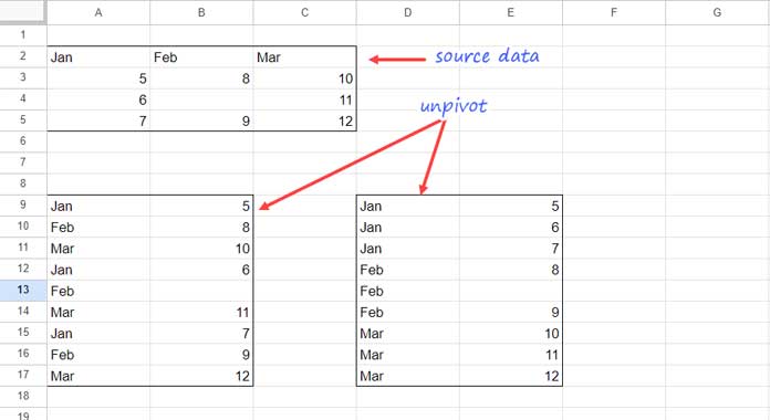
In cell A9, I’ve used:
=ARRAYFORMULA(SPLIT(FLATTEN(A2:C2&"|"&A3:C5), "|"))This unpivots the array A2:C5. We can achieve the same result by replacing FLATTEN with TOCOL:
=ARRAYFORMULA(SPLIT(TOCOL(A2:C2&"|"&A3:C5), "|"))As mentioned, the default arguments in the TOCOL function will produce a FLATTENed output.
The following D9 formula unpivots the data and returns the result in field label (category) order:
=ARRAYFORMULA(SPLIT(TOCOL(A2:C2&"|"&A3:C5, 0, TRUE), "|"))When you want the unpivoted data categorized by field labels, use the TOCOL function with the scan_by_column argument set to TRUE.
TOCOL and WRAPCOLS to Insert a Blank Row After Every Row
There are several ways to insert a blank row after every other row in Google Sheets. Previously, I posted a tutorial on this topic when the TOCOL and WRAPCOLS functions weren’t available.
Here’s a TOCOL and WRAPCOLS combination formula to achieve the same result:
=ARRAYFORMULA(LET(
   col, TOCOL(A2:C5, 0, TRUE),
   IFERROR(WRAPCOLS(TOCOL({col, col/0}, , FALSE), ROWS(A2:C5)*2))
))Note: Replace A2:C5 with your actual data range.
How does this formula work?
- TOCOL Function: The TOCOL function converts the array A2:C5 into a single column:
TOCOL(A2:C5, 0, TRUE)
This transforms the data into one vertical list. - LET Function: The LET function assigns the name col to the output of the TOCOL formula. Wherever col appears, it refers to this result.
{col, col/0}: This creates an array where the second column contains error values. Dividing col by 0 intentionally generates these errors.- Second TOCOL: The second TOCOL function transforms both the col and the error values into a single column again:
TOCOL({col, col/0}) - WRAPCOLS Function: The WRAPCOLS function takes the output from the second TOCOL and wraps it into columns. The number of rows is doubled (
ROWS(A2:C5)*2) to insert the blank rows. - IFERROR: The IFERROR function replaces the error values (from
col/0) with blank cells, creating the blank rows between the original data rows.
This combination of functions efficiently inserts blank rows after every row in the data range.
Additional Tip: TOCOL as an Initial Value in LAMBDA Functions
This technique is intended for advanced users.
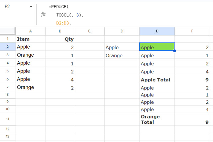
Two LAMBDA functions, REDUCE and SCAN, have an initial value argument. When using REDUCE, it’s common to replace "" (empty string) with TOCOL(, 3).
This serves a key purpose: REDUCE reduces an array to an accumulated result. When you vertically stack the accumulator in each step, if the initial value is an empty string, it leaves an empty cell followed by #N/A. Replacing "" with TOCOL(, 3) eliminates that issue, providing a truly blank value.
For example, suppose column A contains items, and column B contains quantities. The following formula inserts a subtotal between each unique item without leaving an empty row at the top:
=REDUCE(
   TOCOL(, 3),
   D2:D3,
   LAMBDA(a, v,
      VSTACK(
         a,
         VSTACK(
            FILTER(A2:B, A2:A=D2),
            HSTACK(v&" Total", SUM(FILTER(B2:B, A2:A=D2)))
         )
      )
   )
)