If you are one of my regular readers, by now, you may have learned the simplest way to unpivot a dataset, also called reverse pivot, in Google Sheets.
The reason, in one of my earlier posts regarding flattening datasets, one of my readers, Mr. S K Srivastava, has shared this wonderful idea in brief. I am giving due credit to him in this post.
Recently I have posted about the use of an unofficial function in Google Sheets called FLATTEN. We can use this function to unpivot (reverse pivot) a table in Google Sheets.
Must Read: How to Use the FLATTEN function in Google Sheets.
Other than the FLATTEN, we only require SPLIT and the & sign as an ArrayFormula for this.
I’m sure that it’s (the FLATTEN, Ampersand, and SPLIT combo) the simplest way to reverse pivot a table without using Google Apps Script.
Note: If your pivot data is very large like 1000+ rows (it may be very rare), this formula may not work as the SPLIT function has normally an issue with such a large set of data.
The Easiest Way to Unpivot a Dataset in Google Sheets
Sample Data to Reverse Pivot
Here for the example, I am importing a suitable table for our test from this Wiki page using the following IMPORTHTML formula.
Formula:
=array_constrain(
     IMPORTHTML(
        "https://en.wikipedia.org/wiki/International_wheat_production_statistics",
        "table",1
     ),6,5
)
For your info, the Array_Constrain is part of the IMPORTHTML formula to constrain the size of the imported table.
Sample Data Imported:
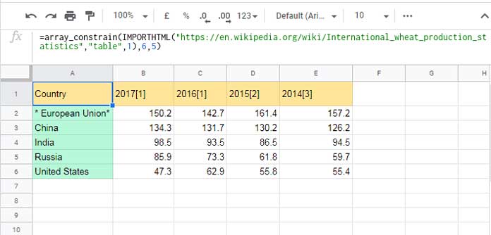
The data shows worldwide wheat production from the year 2014 to 2017. The country names are in column A and year-wise productions are in columns B to E.
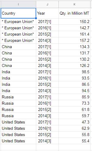
Let’s see how to unpivot the above data in Google Sheets. I mean, country names in the first column, years in the second column, and qty. in the third column as below.
Unpivot Formula in Google Sheets
Below is the simple formula (key in cell I2) to reverse pivot a table in Google Sheets.
Unpivot Formula:
=ARRAYFORMULA(
     split(
        flatten(
           A2:A6&"|"&B1:E1&"|"&B2:E6
        ),"|"
     )
)
If you want field labels like the ones in I2:K2 (please refer to the image above), insert this {"Country", "Year", "Qty. in Million MT"; just after the equal sign in the formula and close the formula with }.
Formula Explanation (How to Use the Formula)
The FLATTEN function is the key. Inside the FLATTEN formula, combined the first column in the range (A2:A6) with the first row in the range (B1:E1) and then combined the rest of the data (B2:E6).
The Pipe sign (you can use any other character like a Tide) is inserted in between to facilitate splitting the flattened combined data.
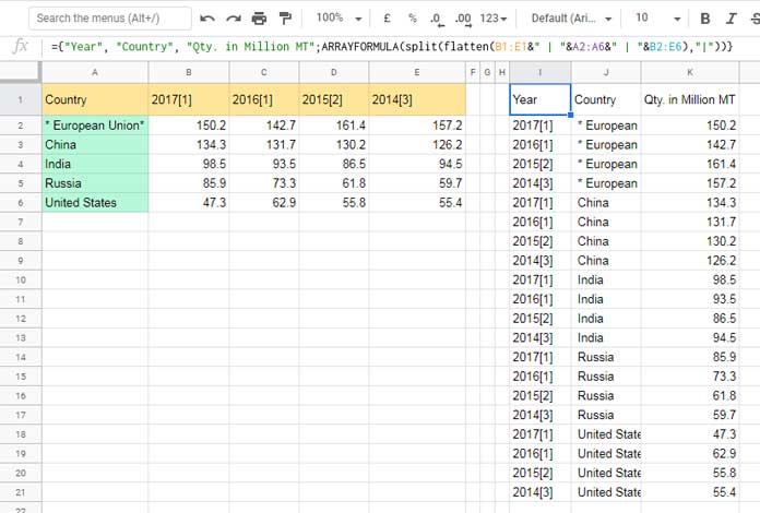
If you want, you can modify the combined range within the FLATTEN like; combine the first row in the range (B1:E1) with the first column in the range (A2:A6) and then the rest of the data (B2:E6).
If you follow this to unpivot the above dataset in Google Sheets, it would look like as below.
Can We Use Open Ranges Instead of Closed Ranges in Flatten?
Using A2:A and B2:E instead of A2:A6 and B2:E6 may cause some issues like #REF! error in the formula, frozen your sheet, or may insert hundreds of blank rows.
Here we can use a technique that I have earlier successfully used with MMULT – Proper Use of MMULT in Infinite Rows in Google Sheets.
What’s that?
Replace A2:A6 with the dynamic (infinite/open) range;
array_constrain(A2:A,MATCH(2,1/(A2:A<>""),1),1)Replace B2:E6 with the dynamic (infinite/open) range;
array_constrain(B2:E,MATCH(2,1/(A2:A<>""),1),4)There are 4 columns in the range B2:E6. The 4 in the last part for the formula represents this total number of columns.
How to Include More Than One Fixed Column in the Unpivot Dataset in Google Sheets?
In the example above, we have only one fixed column and that is column A that contains the ‘Country’.
If we want we can include more than one fixed column in the unpivot dataset in Google Sheets. For that, we must modify the above formula slightly. I have a dynamic way (formula) to do that.
I mean we can include any number of fixed columns with a minor tweak in the reverse pivot formula above.
Here is my new sample data. I’ve included an additional column named ‘Continent’ to our earlier sample dataset (please refer to Image # 01 for the old dataset).
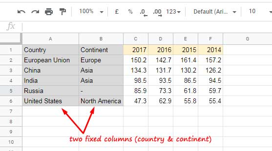
If you skip the ‘Continent’ column B, in line with our earlier reverse pivot formula, the formula (1 fixed column) for this range would be as below.
=ARRAYFORMULA(
     split(
        flatten(
           A2:A6&"|"&C1:F1&"|"&C2:F6
        ),"|"
     )
)
I’ve skipped B2:B6 and as a result, the unpivot output would be similar to Image # 02 above.
Let’s see how to include multiple fixed columns in the unpivot dataset in Google Sheets.
Steps
In the above formula, A2:A6 is our one and only fixed column. But what we want is A2:B6. Replacing A2:A6 with A2:B6 won’t do the trick. Then?
You just use this formula instead of A2:B6. That means you should replace A2:A6 in the just above formula with the below formula that starts with ‘transpose’.
transpose(query(transpose(A2:B6&"|"),,9^9))So the formula to unpivot a dataset with more than one (here two) fixed column would be as below.
Unpivot Multiple Fixed Columns Formula:
=ARRAYFORMULA(
     split(
        flatten(
           transpose(query(transpose(A2:B6&"|"),,9^9))&"|"&C1:F1&"|"&C2:F6
        ),"|"
     )
)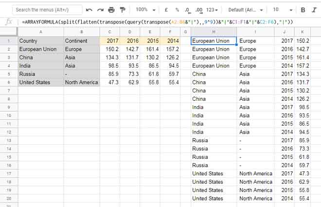
You can now easily make more columns as fixed by changing A2:A6. I mean A2:B6 as above for two columns, A2:C6 for three columns, and so on.
Benefits of Reverse Pivot
The main benefit of reverse pivoting a dataset is that it brings flexibility to manipulate the data with functions like SUMIF, QUERY, FILTER, VLOOKUP, etc.
Here are two examples. Let me start with SUMIF.
Assume we want to calculate the total Wheat production in the country China during the years 2014-2017. We can use the SUMIF as below (data as per Image # 03).
=sumif(J2:J21,"China",K2:K21)Please see the just above screenshot for the range used in SUMIF.
Note: If you use " | " instead of "|" within the unpivot dataset formula, then the above SUMIF would return 0 due to a mismatch of criteria.
In the next example, I am using QUERY to group the countries and total the Wheat production.
=query({I1:K21},"Select Col2, Sum(Col3) group by Col2") Result:
| Country | sum Qty. in Million MT |
| European Union* | 611.5 |
| China | 522.4 |
| India | 373 |
| Russia | 280.7 |
| United States | 221.4 |
Here, you feel free to replace I1:K21 with the unpivot formula itself.
That’s all about how to unpivot a dataset in Google Sheets. Thanks for the stay. Enjoy!
Resources:
- How to Use the GETPIVOTDATA Function in Google Sheets.
- Create Age Analysis Report Using Google Sheet Pivot Table.
- Drill Down Detail in Pivot Table in Google Sheets [Date Grouping].
- How to Format Query Pivot Header Row in Google Sheets.
- How to Pivot Multiple Columns in Query in Google Sheets.
- All About Calculated Field in Pivot Table in Google Sheets.
- How to Sort Pivot Table Grand Total Columns in Google Sheets.
- How to Sort Pivot Table Columns in the Custom Order in Google Sheets.
- Extract Total and Grand Total Rows From a Pivot Table in Google Sheets.
- How to Filter Top 10 Items in Google Sheets Pivot Table.


Hi Prashanth,
Thanks a lot for your post. It helped me a lot and worked well. I can’t thank you enough.
It worked very well until I started receiving files which don’t have all the values filled.
Current Formula:
=ARRAYFORMULA(split(flatten(A2:A11&"|"&B2:B11&"|"&C2:C11&"|"&D1:K1&"|"&D2:K11)
,"|"))
Expected: I don’t want any row which has null in the value columns.
Hi, Ravi,
You can try the below formula.
=query(ARRAYFORMULA(
split(
flatten(A2:A11&"|"&B2:B11&"|"&C2:C11&"|"&D1:K1&"|"&D2:K11)
,"|")),
"Select * where Col5 is not null")
The outer Query will filter out the unwanted rows.
Hi, thank you so much for this article! It is fantastic!
I’m trying to implement something like the final example where there is more than one fixed column, but it is also an infinite range.
When I try to apply the note for the infinite range to the multiple columns concept, it keeps giving me a literal array error. I’m not sure what I’m doing wrong.
Could you show an example formula for the multiple fixed columns with infinite range added?
Hi, Vic,
In my example sheet, in the tab “More than one Fixed Column,” I have added some notes in the range M1:N5. That will guide you in the correct direction.
OMG! THANK YOU SO MUCH! This was exactly what I needed and worked beautifully in my sheet! Can’t thank you enough! This article has saved my team so much work!
Hi, This is really great. I was looking for something like this. Now I have an issue that I have multiple Value fields also.
So my data is like 13 fixed fields, 50 value fields (10 value fields with 5 fields each). You can also see it as a multiple-layer row.
Any solution for that?
Hi, Aayush,
Can you show me a sample of your data and the result you are expecting? I just want 3 fixed fields, 3 value fields, and their sub.
You can leave the URL via comment.
Just here to say it was so helpful and enlightening. Thanks, y’all!
Great solution! Thank you very much!!! I have noticed that some values when unpivoting several fixed columns get a blank space added at the beginning of the string. Looks like it happens to you too. Do you know how to fix it? Thanks!!!!
Hi, Elisa Tormes,
It’s because of the QUERY.
We can solve it by using the TRIM function within the formula as below.
=ARRAYFORMULA(trim(split(flatten(transpose(query(transpose(A2:B6&"|"),,9^9))&"|"&C1:F1&"|"&C2:F6),"|")))
It has one issue though!
Adding TRIM will convert the numeric column into a text column.
In my case, the formula will convert columns J and K in the unpivot data to text columns.
So in such case, if you use those columns in other calculations you should use the VALUE function.
Eg.:
=sum(K1:K20)It won’t work. Use it as
=ArrayFormula(sum(value(K1:K20)))Thank Prashanth! Will definitely try it!
The formula works really nicely! I’m just wondering: is it possible to make the formula remove null entries?
Let’s say for the example you gave above in Image 01, E4 and E5 do not have any values. So I don’t want them showing up in the output. How would you do that?
Hi, Nick,
We can use Query to filter out the blanks in the third column (column 1 contains the country name, column 2 contains years and column 3 contains values).
=Query(ARRAYFORMULA(split(flatten(A2:A6&"|"&B1:E1&"|"&B2:E6),"|")),"Select * where Col3 is not null",0)It took me a while to understand what exactly is happening. Brilliant use of headers option of the Query function.
Thanks.
In real life not more than 3-4 fields are fixed in that case simply use of
"&"as follows should be sufficient=ArrayFormula(SPLIT(FLATTEN(ArrayFormula(A6:A13&"♣"&B6:B13&"♣"&C6:C13&"♣"&D6:D13&"♣"&
amp;E5:H5&"♣"& E6:H13)),"♣",1,0))
Hi, SKS,
I agree with you 🙂
It works really nice. Thanks.
Thank you very much for the update.
I really enjoy your site very much. Keep on the good work.
Kind regards.
Hi, MMC,
Thanks for your feedback!
Thanx for giving credit to me. I appreciate your gesture.
I have further modified the formula to accommodate more than one fixed column.
Hello,
I’m very much interested in a formula to accommodate more than 1 fixed column. Would you be so kind to share it here?
Kind regards.
Hi, MMC,
Updated the post to incorporate the required changes. I also included my (experiment) sheet.