This tutorial introduces one of the simplest and most efficient formulas to stack data in Google Sheets. But first, let’s discuss the benefits of stacked data over unstacked data.
Benefits of Stacked Data:
- A stacked dataset simplifies statistical analysis and modeling.
- It’s suitable for lookup and statistical functions in Google Sheets.
- Summarizing stacked data is straightforward with QUERY or Pivot Table functions, streamlining data processing and analysis.
- Allows for easy comparison of multiple variables.
There isn’t a single formula to stack data in Google Sheets. The approach depends on the structure of your data. Here, I’ll share two different examples of stacking data to give you a general idea of the procedure.
Example 1: Stacking Data with Category and Item Columns
In this example, the header row in cells A1:H1 contains group names (Group A to Group H), and the rows below contain participants in each group.
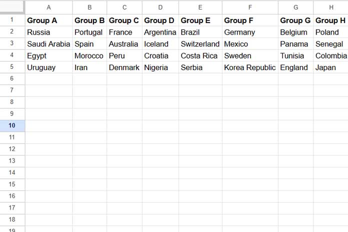
To stack this data, consider the labels in the header row as the category column. Follow these steps:
Note: It’s best to use fixed ranges when stacking data. Here, the header row is in A1:H1, and the data is in A2:H5.
Step 1
In cell K2, enter the following formula:
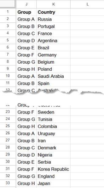
=TOCOL(A2:H5)This formula flattens the range A2:H5 into a single column.
Step 2
In cell J2, enter this formula:
=ArrayFormula(
   TOCOL(
      VLOOKUP(
         SEQUENCE(ROWS(A2:H5), 1, 1, 0),
         HSTACK(1, A1:H1),
         SEQUENCE(1, COLUMNS(A1:H1), 2, 1),
         0
      )
   )
)- Explanation: This step 2 formula repeats the labels from the header row (A1:H1) for each row in the original data (A2:H5), resulting in stacked data with category labels.
Here’s how each part works:
- VLOOKUP Part:
VLOOKUP( SEQUENCE(ROWS(A2:H5), 1, 1, 0), HSTACK(1, A1:H1), SEQUENCE(1, COLUMNS(A1:H1), 2, 1), 0 )search_key:SEQUENCE(ROWS(A2:H5), 1, 1, 0)generates a series of 1s matching the number of rows in A2:A5.range:HSTACK(1, A1:H1)horizontally stacks 1 with the labels in A1:H1.index:SEQUENCE(1, COLUMNS(A1:H1), 2, 1)generates indices from 2 onward, matching the columns in A1:H1.is_sorted: 0 (indicates an unsorted range).
The VLOOKUP searches the generated 1s in the first column of the range and returns values from other columns, effectively retrieving the labels for each row.
- TOCOL Part: This part flattens the category labels returned by the VLOOKUP, aligning them with the stacked data from Step 1.
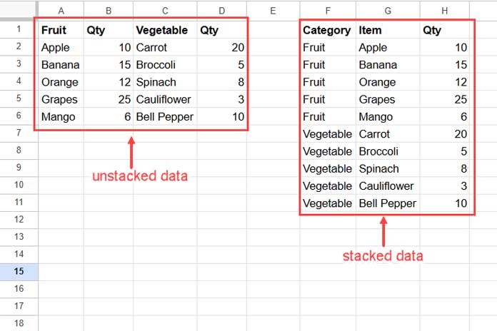
Example 2: Stacking Data with Category, Item, and Quantity Columns
For this example, imagine a table like this:
| A | B | C | D |
| Fruit | Qty | Vegetable | Qty |
| Apple | 10 | Carrot | 20 |
| Banana | 15 | Broccoli | 5 |
| Orange | 12 | Spinach | 8 |
| Grapes | 25 | Cauliflower | 3 |
| Mango | 6 | Bell Pepper | 10 |
The labels “Fruit” and “Vegetable” act as categories, as they each appear once.
Step 1
In cell G2, enter the following formula:
=VSTACK(A2:A6, C2:C6)This vertically appends the ranges A2:A6 and C2:C6.
Step 2
Next, in cell H2, enter:
=VSTACK(B2:B6, D2:D6)This vertically appends the ranges B2:B6 and D2:D6.
Step 3
Now, repeat the labels from A1 and C1 using VLOOKUP. In cell F2, enter:
=ArrayFormula(
   TOCOL(
      VLOOKUP(
         SEQUENCE(ROWS(A2:A6), 1, 1, 0),
         HSTACK(1, A1, C1),
         {2, 3},
         0
      ),,TRUE
   )
)- Explanation:
- The VLOOKUP part is similar to Example 1, but here it returns the category labels “Fruit” and “Vegetable”.
- The TOCOL function then flattens these labels. In this formula, we specify TRUE as the final argument in TOCOL to scan the values by column instead of by row, since vertical stacking of data is done in steps 1 and 2.
Conclusion
In this tutorial, we explored how to stack data in Google Sheets. Since these are individual formulas, sorting the stacked data by category may require an additional SORT formula.
For Example 1, a combined formula could look like this:
=HSTACK(
   ArrayFormula(TOCOL(VLOOKUP(SEQUENCE(ROWS(A2:A5), 1, 1, 0), HSTACK(1, A1:H1), SEQUENCE(1, COLUMNS(A1:H1), 2, 1), 0))),
   TOCOL(A2:H5)
)
This formula follows the general structure: HSTACK(step2_formula, step1_formula).
For Example 2, use:
=HSTACK(
   ArrayFormula(TOCOL(VLOOKUP(SEQUENCE(ROWS(A2:A6), 1, 1, 0), HSTACK(1, A1, C1), {2, 3}, 0),,TRUE)),
   VSTACK(A2:A6, C2:C6),
   VSTACK(B2:B6, D2:D6)
)
This formula follows the general structure: HSTACK(step3_formula, step1_formula, step2_formula).
Wrap these with SORT to sort the stacked columns as needed.
Additional Resources
- How to Unstack Data into Groups in Google Sheets
- Unstack Multiple Form Responses in Google Sheets
- A Simple Formula to Unpivot a Dataset in Google Sheets
- Unpivot Excel Data Fast: Power Query & Dynamic Array Formula
- Split Your Google Sheet Data into Category-Specific Tables
- Dynamic Formula: Split a Table into Multiple Tables in Google Sheets


I’m trying to find something similar to this, but what I need to do is stack three columns on top of each other from separate tabs.
Tab1: (Col A) Product (Col B) Image (Col C) Link
Tab2: (Col A) Product (Col B) Image (Col C) Link
Tab3: (Col A) Product (Col B) Image (Col C) Link
I want to simply stack Tab1, Tab2, and Tab3 on top of each other in Tab4 (because the original tabs need to remain separate) so whenever data is added to any of the first 3 tabs, Tab4 will always update with the cumulative list of everything.
I don’t want to keep headers or anything like that, no sorting required (although removing blanks would be helpful) just stacking one tab on top of the other.
Thanks in advance,
Duncan
Hi, Duncan Rice,
This may help.
Change sheet names (tab names). If returns error, please read How to Change a Non-Regional Google Sheets Formula.
Hello & Questions…
1) How do you add Column Titles to your Stacked Data?
Referring to your Stacking from Unstacked data, there are no column titles in Stacked data
(I guess some might term this: Reverse Pivot or UnPivot)
2) Is there any way to add a column with data? I am Stacking from different spreadsheets and want to add the column to indicate which spreadsheet it came from
You provide wonderful resources and Instruction.
THANK YOU!!
Tony
Hi, Tony,
Glad to hear that you find my tutorials useful.
Regarding column titles, you can try this.
={"Group","Country";QUERY(ArrayFormula(SPLIT(TRANSPOSE(SPLIT(textjoin("-",TRUE,TRANSPOSE((A1:H1&","&A2:H5))),"-")),",")),"Select * where Col2<>''")}Here the column titles are “Group” and “Country”.
Best,