We can group data by month and year in Google Sheets in two ways: using the Pivot Table or using the QUERY function. This tutorial covers both methods, but I give more emphasis to the QUERY function.
Please note that the title includes both the month and year. I intentionally included the year in the title because grouping data by month and year can be helpful in certain situations, such as when you have data to manipulate from multiple years.
Grouping data by month and year allows you to display the month as Jan-2018, which is more informative than simply showing January or month number 1 for the first month of 2018.
In a sales report, if sales transactions occur in different years, grouping data by month alone may cause wrong results. This is because the same month can occur in multiple years, and the data for those months would be added together.
However, if all of the sales transactions occur in the same year, then grouping by month is not a problem.
So, here are my tips to avoid such mistakes in Google Sheets. For our explanation, I will be using a sample diesel consumption report.
Suppose I have two heavy vehicles and I have recorded the diesel consumption of these vehicles by date. I can use this data to create a month- and year-wise summary report.
Once you have learned this Google Sheets month and year grouping technique, you can use it to group different types of datasets, such as sales reports, purchase orders, and material reconciliations.
How to Group Data by Month and Year in Google Sheets with Pivot Tables
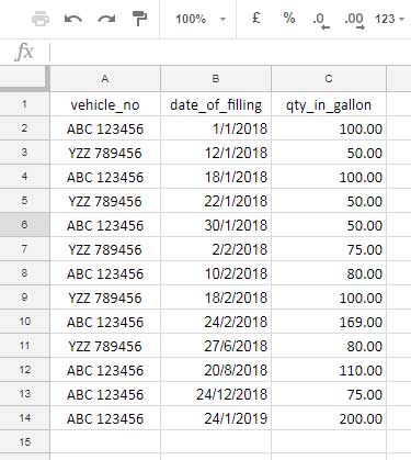
We will use the following diesel consumption data for our example. You can type it as it is or copy it from my example sheet at the end of this tutorial.
The data contains 13 vehicle numbers in column A (not unique), the date of fuel filling in column B, and the quantity in gallons in column C.

Steps to create a month- and year-wise summary using a Pivot Table from this data in Google Sheets:
- Select the data range A1:C14.
- Go to the Insert menu and click Pivot Table.
- In the Pivot Table dialog box, select the Existing sheet option and enter E1 in the Location field. Click Create.
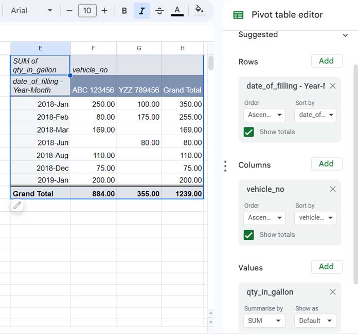
- In the Pivot Table editor pane, drag the date_of_filling field to the Rows area.
- Drag the vehicle_no field to the Columns area.
- Drag the qty_in_gallon field to the Values area.
- Right-click on any value in column E in the Pivot Table, and select Create Pivot date group > Year-month.

That’s it!
This will create a Pivot Table that summarizes the data by month and year.
Just a quick reminder: when creating a Pivot Table, make sure to select the actual data range, here A1:C14.
If you do select the entire columns, here A1:C, you may need to filter the table to remove blank rows. To do this, simply head to the Filters section located under Values in the Pivot Table editor and add the desired column(s) to the filter.
How to Group Data by Month and Year in Google Sheets with QUERY Function
Now see the formula to group data by month and year in Google Sheets. The formula explanation follows just after that.
Master Formula:
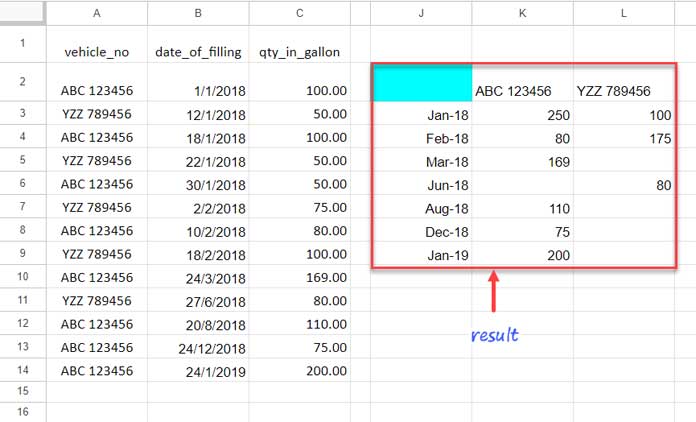
=QUERY(HSTACK(A2:A14,ARRAYFORMULA(EOMONTH(B2:B14,0)),C2:C14),"SELECT Col2,SUM(Col3) GROUP BY Col2 PIVOT Col1 FORMAT Col2'MMM-YY'")
Notes:
- In the QUERY formula, the column identifiers are case-sensitive. So, you must specify them as
Colinstead ofCOLfollowed by the column number. - The above formula is for the range
A2:C14. If you use it for the rangeA2:C, you must use the formula as follows:
=QUERY(HSTACK(A2:A,ARRAYFORMULA(IFERROR(EOMONTH(DATEVALUE(B2:B),0))),C2:C),"SELECT Col2,SUM(Col3) WHERE Col1 IS NOT NULL GROUP BY Col2 PIVOT Col1 FORMAT Col2'MMM-YY'")Formula Explanation: Month-Wise Grouping of Data Across Different Years
As you can see above, I have used a QUERY formula for this purpose. I previously shared a similar tutorial on how to sum by month in Google Sheets. It used the SUMIF function, but it only works for a specific year. If the data spans multiple years, the formula may not work.
I also posted another tutorial on how to create a month-wise summary in Google Sheets using the QUERY formula. However, that formula also has the same issue. You can only use it for dates that fall within a single year.
Therefore, I would like to draw your attention to my above QUERY formula for grouping data by month and year in Google Sheets. This formula works regardless of whether the data spans multiple years.
Although QUERY is the main function used in the formula, the core essence of the formula is the EOMONTH function. I’ll explain why.
In our master formula, instead of using the range A2:C, I have used a customized array range as follows.
HSTACK(A2:A,ARRAYFORMULA(IFERROR(EOMONTH(DATEVALUE(B2:B),0))),C2:C)We have appended the ranges A2:A, B2:B, and C2:C using the HSTACK function. Also, the range B2:B has been replaced by an array formula, which is as follows.
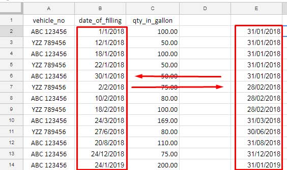
ARRAYFORMULA(IFERROR(EOMONTH(DATEVALUE(B2:B),0)))If you apply this formula in the first cell of any blank column, you will see that it replaces the dates in column B with the end-of-the-month dates.
For example, the date in cell B2 is 1/1/2018. This formula converts this date to 31/1/2018.
It is applicable to all dates in column B. See this screenshot to understand the conversion. In cell E2, I have applied the above EOMONTH formula to show you the output.
Note: Formatted E2:E to dates (Format > Number > Date).

The Advantage of Converting Date to End of Month Date in Google Sheets Formula:
The advantages of this conversion are as follows:
- Instead of having assorted dates in a month, we have common end-of-the-month dates. For example, any date in January 2018 will be converted to 31/01/2018, any date in February 2018 will be converted to 28/02/2018, and so on.
- This allows us to group the data based on these end-of-the-month dates, which can act as a month-wise grouping. We can then format these end-of-the-month dates to show the month and year.
If you understand the above EOMONTH concept, learning the rest of the QUERY formula will be easy for you.
In the Pivot Table, we used the date_of_filling (column 2) in the Rows section and the vehicle_no (column 1) in the Columns section for grouping. Please scroll up and see Figure 2.
The equivalent in the QUERY formula is to group the data by column 2 and pivot by column 1.
"SELECT Col2,SUM(Col3) WHERE Col1 IS NOT NULL GROUP BY Col2 PIVOT Col1 FORMAT Col2'MMM-YY'"I have formatted the end-of-the-month dates to month and year by using the format clause in Query.
This way, you can use the QUERY formula to group data by month and year in Google Sheets.
Conclusion
The above QUERY formula has the following peculiarities:
It groups data by month and year, not just by month. This means that if any date falls in the same month but in different years, there will be an individual month-wise total for each year. For example, 01/01/2017 and 01/01/2018 will be grouped as Jan-2017 and Jan-2018 separately.
The summary retains the month and year order. This is one of the big advantages of this month and year-wise grouping formula. If you use any other formula to group by month, where text formatting is applied, it won’t retain the month and year order. It may sort based on alphabetical order.
We can create a pivot chart from the above QUERY formula. You can also use a PivotChart from the Pivot table, but only with a workaround.


Wow, amazing article. Really helps me to do it. Very well explained. Thanks for it.
Hi,
How do we refer to the columns if we want to build the query on a different tab?
Thank you.
Hi, Anh,
Just include the tab name with the data. E.g.,
query(Sheet10!A1:Jinstead ofquery(A1:JThere are no changes in column reference.
Thanks a lot for this Tuto, I think it can be really powerful in many situations
As a side note:
I’ve spending 2h to figure out why the formula wasn’t working, before discovering that in foreign countries than US, for the curly brackets we we wouldn’t use the “,” but “\” instead, and for all general “,” we use the “;” instead.
As they always make difference between Mac and Windows (cmd and ctrl), I think it woud be great to add a small note in your tutos explaining which caracter should be replaced for foreign countries
Best regards
Hi, Tristan,
I am glad that you liked the tutorial. I have already a tutorial on the locale settings.
How to Change a Non-Regional Google Sheets Formula
I´m trying to use the formula, but it says than “I´m missing one on more close parenthesis”, could you advise on this?. thanks!
Hi Luis,
I’ve tested the formula again and it’s perfect.
But I’ve updated my post. Earlier I was entering formulas in my posts as a blockquote. So the copied formula may not work on your sheet.
Nowadays I’m updating my all the posts one by one with changing the blockquote to “code”. I’ve just updated this post.
Now please copy the formula again and it may work.
Hope this may solve your problem.
Very nice. I’ve been wondering how to do this for a long time.