The EOMONTH function in Google Sheets helps users find the last day of a month before or after a specified date. It can be effectively combined with other date functions, such as WEEKDAY, WORKDAY, SEQUENCE, and QUERY, to extend its functionality.

What is its Role?

The EOMONTH function returns the last day of the month that is n months before or after a given date.

For instance, if you want to generate dates for a Gantt chart, you could use the EOMONTH function to create a range of dates representing the entire project timeline.

Complex Use Cases

• With SEQUENCE: You can generate a full year of month-end dates, which can serve as row headers in your data.
• With QUERY: While QUERY can group a date column by month number, using EOMONTH allows grouping by month text.
• With WORKDAY: Use EOMONTH in conjunction with WORKDAY or WORKDAY.INTL to find the first or last working day of a given month.
• With WEEKDAY: Identify a specific day of the week at the end of the month.

And many more…

Syntax and Arguments

Syntax: EOMONTH(start_date, months)

Arguments:

• start_date: The date from which to calculate the last day of the month.
• months: The number of months to add or subtract from start_date. Use a positive number to find a future month and a negative number for a past month.

Tip: Enter 0 to find the end of the month for the specified date, 1 for the end of the following month, and -1 for the end of the previous month.

Example:

If cell A1 contains the date January 1, 2023, the formula =EOMONTH(A1, 11) in cell B1 will return December 31, 2023.

Conversely, =EOMONTH(A1,-13) in cell C1 will return December 31, 2021.

Generating End-of-Month Dates Using a Date, Month Number, or Month Text

The EOMONTH function is designed to return the last day of a month based on a specific date. However, you can also adjust it to derive month-end dates from a month text or month number. Here are some examples:

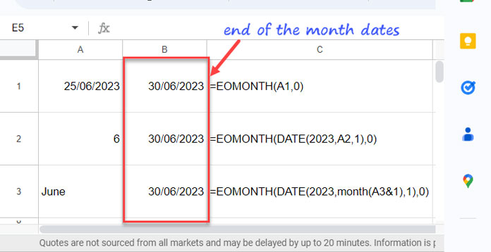
End of the Month Date from a Date:

=EOMONTH(A1, 0)

End of the Month Date from a Month Number:

=EOMONTH(DATE(2023, A2, 1), 0)

Note: The DATE function combines a specified year, month, and day into a date. Its syntax is:
DATE(year, month, day)
In this formula, you specify the year (2023 in this case), the month (from cell A2), and the day (set to 1 to represent the first day of that month). The EOMONTH function then returns the last day of the specified month.

End of the Month Date from a Month Text:

=EOMONTH(DATE(2023, MONTH(A3 & 1), 1), 0)

How to Get the First Day of a Month in Google Sheets

You can use the EOMONTH function to determine the last day of a month. By supplying a negative value for the ‘months’ argument, such as -1, the function will return the last day of the previous month. You can then add 1 to this date to find the first day of the current month.

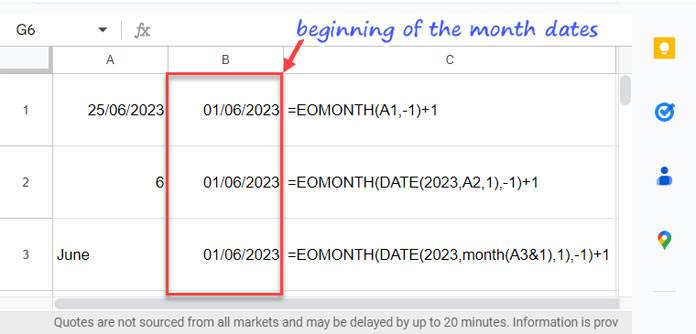
1. Month Start Date from a Date:
   =EOMONTH(A1, -1) + 1
2. Month Start Date from a Month Number:
   =EOMONTH(DATE(2023, A2, 1), -1) + 1
3. Month Start Date from a Month Text:
   =EOMONTH(DATE(2023, MONTH(A3 & 1), 1), -1) + 1

EOMONTH Function with SEQUENCE in Google Sheets

When creating a Gantt chart or KPI dashboard, you might need a header row with month names. Instead of manually entering month names, you can generate month start dates and format them to appear as month text. For example, if cell A1 contains the title “Name” and cells B1:M1 are designated for months, use the following formula in cell B1:

=ARRAYFORMULA(EOMONTH(DATE(2023, 1, 1), SEQUENCE(1, 12,-1)) + 1)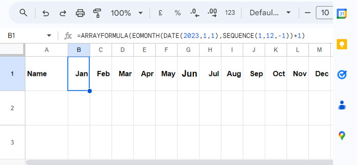

How This Formula Works

• DATE(2023, 1, 1) returns January 1, 2023, as the starting date.
• SEQUENCE(1, 12, -1) generates an array of numbers starting from -1 up to 10, representing the ‘months‘.
• EOMONTH returns the last day of the month based on the sequence. Starting from -1 ensures the month-end dates are from the previous months.
• +1 adjusts the end dates to the first day of each month.

You can format these cells to display month names while retaining the underlying date values.

Formatting Steps:

1. Select cells B1:M1.
2. Go to Format > Number > Custom number format.
3. In the Type field, enter mmm and click Apply.

EOMONTH Function with WEEKDAY in Google Sheets

In a previous tutorial, I discussed how to find the date of the last Saturday of a given month using the EOMONTH function with the WEEKDAY function. Here’s a generalized formula to find any last weekday or weekend of a specified month.

Steps:

1. In a cell (for example, B2), enter the start date of the month (e.g., 1/12/2023) or any date.
2. In cell C2, insert the following formula to find the last Sunday:

=TO_DATE(LET(wd, 1, dt, SEQUENCE(7, 1, EOMONTH(B2, 0), -1), FILTER(dt, WEEKDAY(dt) = wd)))

To find the last Monday, replace 1 with 2 (the corresponding weekday number). The weekdays correspond to:

1: Sunday
2: Monday
3: Tuesday
4: Wednesday
5: Thursday
6: Friday
7: Saturday

For the last Friday in a given month, use:

=TO_DATE(LET(wd, 6, dt, SEQUENCE(7, 1, EOMONTH(B2, 0), -1), FILTER(dt, WEEKDAY(dt) = wd)))

Formula Breakdown

• SEQUENCE: SEQUENCE(7, 1, EOMONTH(B2, 0), -1) returns a sequence of dates starting from seven days before the month-end date.
• FILTER: Filters the dates returned by SEQUENCE to include only those matching the specified WEEKDAY number.
• LET: Names the SEQUENCE output as dt and the weekday number as wd for easier reference.

The Role of EOMONTH in QUERY

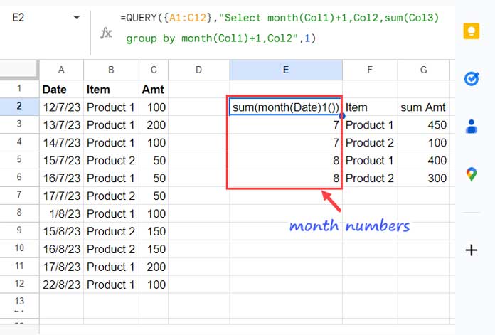
The EOMONTH function is particularly useful in the QUERY function in Google Sheets for grouping date columns by month or by month and year. Although QUERY does not strictly require EOMONTH for grouping, it typically uses month numbers, which can be limiting.

Example QUERY Formula

=QUERY({A1:C12}, "SELECT MONTH(Col1) + 1, Col2, SUM(Col3) GROUP BY MONTH(Col1) + 1, Col2", 1)

This formula sums column C (Col3) by grouping column A (Col1) by month and column B (Col2) by item. The +1 is necessary because QUERY returns month numbers starting from 0 (January = 0).

Using EOMONTH with QUERY

To incorporate EOMONTH in your QUERY, follow these steps:

1. Convert dates in A2:A12 to the beginning of the month:
   =ARRAYFORMULA(EOMONTH(A2:A12, -1) + 1)
2. Append the converted dates with items and amounts:
   ={ARRAYFORMULA(EOMONTH(A2:A12, -1)+1), B2:C12}
3. Use the formula as follows:

=QUERY({ARRAYFORMULA(EOMONTH(A2:A12,-1)+1), B2:C12},"SELECT Col1, Col2, SUM(Col3) GROUP BY Col1, Col2 FORMAT Col1 'mmmm-yy' ",0)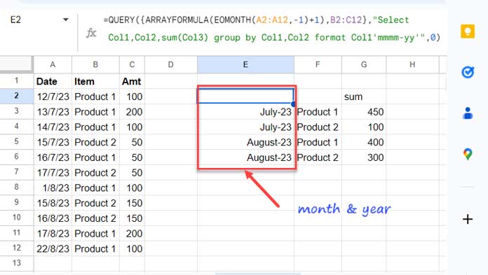

EOMONTH Function with WORKDAY in Google Sheets

In a previous post, I demonstrated how to use the EOMONTH function with the WORKDAY.INTL function to find the first and last workdays of a month (refer to the resources below). In most cases, you can use the WORKDAY function instead of WORKDAY.INTL.

Resources

• Finding the First and Last Workdays of a Month in Google Sheets
• How to Find the Last Business Day of a Month in Excel
• Google Sheets: The Complete Guide to All Date Functions