Getting a Google Sheets formula parse error after copying a formula from a website, tutorial, or forum?
There are two main reasons this happens: a regional separator mismatch or invalid characters.
Quick Fix for Google Sheets Formula Parse Error
If you copied a formula from a US or UK tutorial but your spreadsheet uses an EU or Latin American locale (like France, Germany, or Spain), you simply need to swap your formula separators based on the rules below:
| Element | US / UK Locale | EU / Latin America Locale |
|---|---|---|
| Formula Delimiter | Comma ( , ) | Semicolon ( ; ) |
| Horizontal Array | Comma ( , ) | Backslash ( \ ) |
| Vertical Array | Semicolon ( ; ) | Semicolon ( ; ) |
⚠️ Important Check: Always ensure that all double quotes, commas, and semicolons in your formula are standard, plain-text characters—not stylized or “curly” punctuation copied from a webpage. Additionally, if you are building an inline array using curly braces, double-check that you haven’t accidentally typed a closing parenthesis like { ) instead of the correct closing curly bracket { }.
Following these syntax formatting rules will ensure your formula parse error goes away instantly!
How Regional (Locale) Settings Trigger Formula Parse Errors
Google Sheets formulas are directly tied to your spreadsheet’s regional settings.
In countries where a comma is used as the standard decimal separator (such as €1,50 instead of $1.50), Google Sheets automatically replaces the standard formula comma with a semicolon to avoid confusion.
US/UK-Style Formula (Period Decimal)
=SUM(A1, B1, C1)European/Latin American-Style Formula (Comma Decimal)
=SUM(A1; B1; C1)If you paste a formula using the wrong regional format into your spreadsheet, Google Sheets will usually try to interpret the formula and convert the operators automatically. However, this automatic conversion can fail—especially with nested functions or arrays. When it fails, you are hit with the dreaded Formula parse error.
Exceptions to the Rule: The QUERY Function Trap
The QUERY function behaves uniquely when adapting formulas to a different locale. It is one of the most common places where users run into unexpected errors because it mixes native spreadsheet settings with its own internal query language.
To see this in action, let’s look at the basic syntax across two different locales:
- UK Locale:
QUERY(data, query, [headers]) - Spain Locale:
QUERY(data; query; [headers])
While the outer function arguments change from a comma to a semicolon, the column identifiers inside the select string must always use a comma, regardless of your locale.
Example 1: Standard Column Selection
Notice how the outer argument separators change, but the column commas inside the quotation marks stay exactly the same:
UK Locale (Comma):
=QUERY(A1:D, "select A, B, sum(C) where A is not null group by A, B", 1)Spain Locale (Semicolon)
=QUERY(A1:D; "select A, B, sum(C) where A is not null group by A, B"; 1)Example 2: Using Worksheet Functions Inside a Query String
The trap deepens when you use a native Google Sheets function (like TEXT) concatenated inside the query string. The internal function must follow your local worksheet rules, while the main QUERY structure adapts around it:
UK Locale:
=QUERY(A1:D, "select A, B where D=date '"&TEXT(E2, "yyyy-mm-dd")&"' ", 1)Spain Locale:
=QUERY(A1:D; "select A, B where D=date '"&TEXT(E2; "yyyy-mm-dd")&"' "; 1)💡 Takeaway: When translating a QUERY formula, only change the punctuation that is outside the literal query string text, unless you are working with an inline worksheet function like TEXT or IF embedded within the cell references.
How to Change Formula Separators in Google Sheets
There are two highly effective ways to adapt a formula to your local spreadsheet settings.
Method 1: Use Find and Replace (Manual Update)
If you only have one or two formulas to fix, you can swap the characters manually using the built-in Find and Replace tool.
- Copy and paste the formula into your cell.
- Press Ctrl + H (Windows) or Cmd + Shift + H (Mac) to open the Find and Replace dialog box.
- In the Find field, enter a comma (
,). In the Replace with field, enter a semicolon (;)—or vice versa, depending on your needs. - Crucial Step: Check the box that says “Also search within formulas”.
- Click Replace All.
⚠️ Proceed with Caution: This tool will replace every single comma in your formula. This can accidentally break your data in two ways:
- Text Criteria: It will alter commas inside text strings (for example,
="Apple, Orange"would turn into="Apple; Orange"). - The QUERY Function Trap: It will mistakenly replace the commas separating your column IDs inside a query string (for example,
"select A, B"will incorrectly change to"select A; B").
Always review your formulas afterward to ensure your text strings and query clauses didn’t change!
Method 2: Change the Spreadsheet Locale (The Automatic Translation Trick)
If you are importing a massive, complex formula or frequently copy work from US/UK tutorials, letting Google Sheets handle the translation automatically is the safest and easiest route.
- Open Settings: Open your spreadsheet and navigate to File > Settings in the top menu.
- Switch to a Comma-Based Locale: Under the General tab, find the Locale dropdown. Change it to a region that natively uses comma separators, such as the United Kingdom or United States. Click Save and reload.
- Paste Your Formula: Paste your copied US/UK formula into the cell. Because the spreadsheet matches the tutorial’s region, the formula will execute perfectly without any errors.
- Revert to Your Home Locale: Go back to File > Settings, change the Locale back to your actual home country, and click Save and reload once more.
Google Sheets will run its background translation and automatically switch all the commas, semicolons, and array brackets to your local format without breaking anything!
How Locale Settings Impact Inline Array Creation
You can build custom arrays in Google Sheets by enclosing cell ranges inside curly braces {}. This is a powerful way to stack data without complex functions.
However, the characters you use to separate the elements within those brackets completely shift depending on your regional settings.
For example, take a look at this standard US/UK-style formula:
=XLOOKUP(A1, {1, 2, 3, 4, 5, 6, 7}, {"Su", "M", "Tu", "W", "Th", "F", "Sa"})If you copy and paste this exact formula into an EU-locale spreadsheet, it will instantly trigger a Formula parse error. This happens because both the function arguments and the internal array lists are using commas.
To fix it for an EU locale, you must change the function commas to semicolons, and the array commas to backslashes:
=XLOOKUP(A1; {1\ 2\ 3\ 4\ 5\ 6\ 7}; {"Su"\ "M"\ "Tu"\ "W"\ "Th"\ "F"\ "Sa"})1. UK / US Locale Settings
In a comma-decimal region like the US or UK, the layout rules are straightforward:
- Horizontal Stack (Side-by-Side / HSTACK): Use a comma (
,) to join ranges horizontally. - Vertical Stack (On Top of Each Other / VSTACK): Use a semicolon (
;) to join ranges vertically.
Array By Row (Horizontal)
={B2:C4, E2:F4}Array By Column (Vertical)
={B2:C4; E2:F4}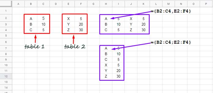
2. Spain / EU Locale Settings
In regions like Spain, France, or Germany where a comma is already used as a numerical decimal point, things change. To prevent syntax confusion, the horizontal separator shifts to a backslash ( \ ), while the vertical separator remains a semicolon:
- Horizontal Stack (Side-by-Side / HSTACK): Use a backslash (
\). - Vertical Stack (On Top of Each Other / VSTACK): Use a semicolon (
;).
Array By Row (Horizontal)
={B2:C4\ E2:F4}Array By Column (Vertical)
={B2:C4; E2:F4}💡 Keep in Mind: If you are using standard modern functions like HSTACK or VSTACK instead of standard curly braces, you don’t need to worry about backslashes. You will just follow the standard regional rules we covered earlier: commas for the UK/US and semicolons for the EU.
Conclusion
Adapting a Google Sheets formula from another region doesn’t have to result in a frustrating #ERROR!. In summary, here are the key takeaways to keep in mind when converting a non-regional formula to your local spreadsheet settings:
- Swap Function Delimiters: Change argument separators from a comma (
,) to a semicolon (;), or vice versa, depending on your region’s decimal format. - The QUERY Exception: Punctuation inside a literal
QUERYstring always uses commas to separate column identifiers, regardless of your locale. However, any nested worksheet function used within that query string must follow your local format. - Array Layout Separators: When building inline arrays with curly braces
{ }, swap the horizontal row separator from a comma (,) to a backslash (\) if you are moving between US and EU locales. - Scrub Hidden Typos: Always look out for non-standard characters like “curly” typographical quotes (
“ ”) or foreign punctuation characters that often slip in when copy-pasting from online forums. - The Shortcut: When in doubt, temporarily change your spreadsheet’s locale in File > Settings, paste your formula, and switch it back to let Google Sheets handle the translation for you automatically.


