While the TRANSPOSE function is a powerful tool for swapping rows and columns in Google Sheets, it’s not the only option. You can also achieve this using:
- Transpose command: Similar to TRANSPOSE, offering enhanced control through copy-paste options.
- TOCOL and TOROW functions: Convert specific rows or columns to new columns or rows, respectively.
Each approach has its strengths and weaknesses, making them suitable for different situations.
This tutorial focuses on the TRANSPOSE function to explore its capabilities in depth, but will also briefly touch upon the other methods for a complete understanding.
TRANSPOSE Function: Syntax, Arguments, and Key Use Cases
Syntax:
TRANSPOSE(array_or_range)Arguments:
array_or_range: The array or range of cells containing the data you want to transpose. This can be a single cell, a range of cells, or even a named range.
When you alter the data orientation from rows to columns or vice versa, the following visual changes occur: The nth column becomes the nth row, and the nth row becomes the nth column.
For instance, the third column transforms into the third row, and vice versa. Applying TRANSPOSE twice maintains the original orientation.
Use Cases:
- Data manipulation: Transposing data can help rearrange your data for easier analysis, such as filtering rows by column values or vice versa. It allows you to work with your data on a different axis.
- Data Presentation: It provides flexibility in how data is presented, making it easier to create Charts or Pivot Table reports.
- Formatting QUERY Pivot headers:
- This is a more advanced tip for QUERY users. If your QUERY Pivot data has dates in the top row and you want to format them as Month, Year-Month, or Year, within the QUERY formula:
- Move the date column to the GROUP BY clause instead of the PIVOT clause.
- Format the date column for your desired display using the FORMAT clause.
- You can then transpose the resulting data using the TRANSPOSE function if needed.
- You can find a tutorial on formatting QUERY Pivot header rows here: How to Format Query Pivot Header Row in Google Sheets.
- This is a more advanced tip for QUERY users. If your QUERY Pivot data has dates in the top row and you want to format them as Month, Year-Month, or Year, within the QUERY formula:
Example of TRANSPOSE Function in Google Sheets and Comparison with the Transpose Command
Example Data:
In the table below, data is initially arranged in columns.
| Emp ID | 100 | 101 | 102 | 103 | 104 | 105 |
| Department | HR | Accounts | Fire & Safety | Industrial Safety | Marketing | Admin |
Changing Data Orientation:
To change the orientation from columns to rows, you can use either the TRANSPOSE function or the “Transpose” command in Google Sheets.
Transposed Table:
| Emp ID | Department |
| 100 | HR |
| 101 | Accounts |
| 102 | Fire & Safety |
| 103 | Industrial Safety |
| 104 | Marketing |
| 105 | Admin |
Using TRANSPOSE Formula:
If the initial data is in the cell range A1:G2, you can use the formula:
=TRANSPOSE(A1:G2)Using Transpose Command:
- Copy the data in the range A1:G2.
- Right-click on any cell outside the range of A1:G2 to open the context menu.
- Select “Paste Special” > “Transposed”.
You can also use a Google Sheets keyboard shortcut in this case.
- Windows: Ctrl + C to copy the selected range, and Alt + E + S + E to apply the paste transposed.
- Mac: Command + C to copy the selected data, and Control + Option + E + S + E to apply the paste transposed.
Choosing Between TRANSPOSE Function and Transpose Command
Consider the pros and cons of each method before choosing:
TRANSPOSE Function:
- Source Update: Changes in the source array are reflected in the transposed array.
- Formatting: This does not retain formatting from the source data.
- Editing: The result cannot be directly edited; the formula will break.
Transpose Command:
- Source Update: Updates in the source array won’t be reflected in the transposed data.
- Cell Formatting: Preserves formatting, including cell color, bold, italics, etc.
- Editing: The transposed data can be directly edited without affecting the source.
Nesting TRANSPOSE Functions
As mentioned earlier, transposing data, performing manipulations, and then transposing again is a common practice in Google Sheets. When doing this, it’s crucial to avoid transposing the initial column or row containing labels.
Let’s say we want to sort the data in A1:G2 by departments using the SORT function. Since we can sort data by columns, not by rows, and the department data is in the second row, we need to transpose the range B1:G2, perform sorting, and then transpose it back.
In addition to that, you can use the HSTACK function to join the labels in the original table with the new table.
Formula:
=HSTACK(A1:A2, TRANSPOSE(SORT(TRANSPOSE(B1:G2), 2, 1)))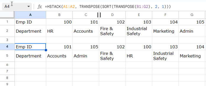
Formula Explanation
The above nested TRANSPOSE formula can be broken down into four parts: Inner Transpose, Sorting, Outer Transpose, and Stacking.
Inner Transpose (TRANSPOSE(B1:G2)):
The innermost TRANSPOSE function transposes the rows and columns of the original data in the range B1:G2.
Sort (SORT(…, 2, 1)):
The SORT function is then applied to the transposed data to sort the ‘Department’ field.
Outer Transpose (TRANSPOSE(…)):
Another TRANSPOSE function is applied to the sorted data. This transposes the sorted data back to its original orientation.
HSTACK (HSTACK(A1:A2, …)):
The HSTACK function horizontally stacks the data in the cell range A1:A2 (labels) and the transposed, sorted data obtained from the previous steps.
TOCOL and TOROW: Alternatives for Single-Row/Column Transposition in Google Sheets
While TRANSPOSE is a versatile tool for swapping rows and columns, TOCOL and TOROW offer alternative approaches for dealing with single-row or single-column data.
In the transposition perspective, you can use these functions with a single column or row, as they are originally designed to transform an array or range of cells into a single column or row.
These functions can ignore blank cells and errors, making them ideal for cleaning data before further analysis.
- TOCOL: Use it to transform one-dimensional horizontal data into vertical data.
- TOROW: Use it to transform one-dimensional vertical data into horizontal data.
Example:
Suppose you have data in A1:A10 with blanks and errors. Experiment with the following formulas to alter the orientation.
=TOROW(A1:A10, 3) creates a new row, skipping blanks and errors.
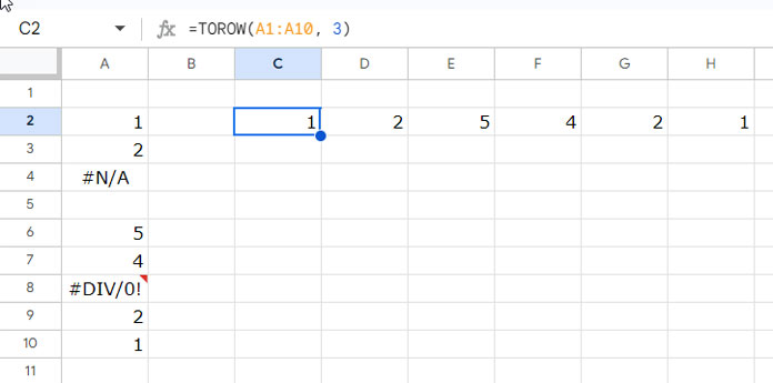
=TRANSPOSE(A1:A10) creates a new row with all data, including blanks and errors, which might not be desirable.
Additional Tips
The TRANSPOSE function typically doesn’t require ARRAYFORMULA support. However, you may encounter examples combining these, and the formula might fail if you remove the latter function.
This occurs when you’re using an expression within the TRANSPOSE function rather than a physical range. The expression requires ARRAYFORMULA support to expand.
For instance, consider a scenario involving SPLIT. You want to split a comma-delimited string and transpose it.
=TRANSPOSE(SPLIT("Apple, Orange, Mango", ","))The above formula will split the text and change the orientation from a single row to a single column.
However, this may leave some space characters with each split text. To address this, you can use TRIM with the above combination.
=ARRAYFORMULA(TRANSPOSE(TRIM(SPLIT("Apple, Orange, Mango", ","))))In this case, you need the ARRAYFORMULA because TRIM requires it to return multiple values.
Common Errors
Here are the two most common errors that you may encounter when working with the TRANSPOSE function in Google Sheets:
1. #REF! Error
- Cause: This error occurs when the reference to the source range is broken.
- Solution: Double-check your formula and ensure the source range still exists in the expected location.
2. #N/A Error
- Cause: This error indicates that TRANSPOSE received more than one range as input. It can only handle a single range or a single cell as the source data.
- Solution:
- Review your formula and ensure you’re referencing only one range, not multiple ranges separated by commas or other operators.
- If you need to combine data from multiple ranges for transposition, consider using nested functions or other approaches to create a single input range.
I hope the information above helps you troubleshoot errors related to this function.


Is there a way to take data in multiple cells like:
e
C c C c
D d d
(each letter in its own cell)
and transform it into one horizontal line (each letter still in its own cell) like:
e C c C c D d d
?
Hi, Caitlin,
Yes! Use TEXTJOIN and SPLIT. I am assuming your sample is in A1:D3. Then the formula (TEXTJOIN and SPLIT) will be;
=split(textjoin("|",1,A1:D3),"|")