
Sometimes you may need to sort Pivot Table rows in a custom order in Google Sheets. Standard alphabetical sorting doesn’t always work for workflows such as sales pipelines, project priorities, task stages, or even month labels.
Google Sheets Pivot Tables don’t include a built-in Custom List feature for sorting row or column labels. That’s understandable because the required order can vary from one workflow to another.
In this tutorial, you’ll learn a dynamic workaround using a helper column to sort Pivot Table rows in any custom order. I’ll also show you how to clean up the Pivot Table layout after applying the sort.
Sample Data and Purpose
Make a copy: Make a copy of the Google Sheets file used in this tutorial.
For this example, we will use the following sample sales pipeline data:
| Deal Name | Sales Rep | Stage | Deal Value |
|---|---|---|---|
| Project Alpha | Varun | Proposal | 15,000 |
| Project Beta | Mike | Qualification | 5,000 |
| Project Gamma | Keerthi | Won | 25,000 |
| Project Delta | David | Negotiation | 12,500 |
| Project Epsilon | Ashish | Qualification | 8,500 |
| Project Zeta | Varun | Won | 45,000 |
| Project Eta | Mike | Proposal | 22,000 |
The sample data is in the range A1:D8.
Our goal is to create a Pivot Table that summarizes Deal Value by Stage and sorts the stages in a workflow-specific order instead of alphabetically.
Default vs. Custom Sort Order
By default, Google Sheets sorts the Stage row labels alphabetically. The following Pivot Table shows the default sort order.
| Stage | SUM of Deal Value |
|---|---|
| Negotiation | 12,500 |
| Proposal | 37,000 |
| Qualification | 13,500 |
| Won | 70,000 |
| Grand Total | 133,000 |
Instead, we want the stages to appear in this custom workflow order.
| Stage | SUM of Deal Value |
|---|---|
| Qualification | 13,500 |
| Proposal | 37,000 |
| Negotiation | 12,500 |
| Won | 70,000 |
| Grand Total | 133,000 |
Let’s proceed with the steps to create the Pivot Table, add a helper column, and sort the Stage field in this custom order.
Step 1: Create the Dynamic Sort Index
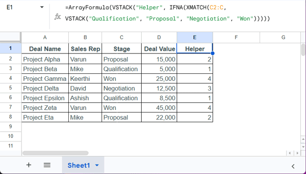
Enter the following formula in cell E1, the header of an empty column next to the dataset:
=ARRAYFORMULA(
 VSTACK("Helper",
   IFNA(XMATCH(
     C2:C,
     VSTACK("Qualification", "Proposal", "Negotiation", "Won")
   ))
 )
)
In the formula:
C2:Cis the Stage column.VSTACK("Qualification","Proposal","Negotiation","Won")defines the required custom sort order.XMATCHreturns the position of each stage in that list, producing a numeric sort index.
The helper column returns:
- Qualification → 1
- Proposal → 2
- Negotiation → 3
- Won → 4
The Pivot Table uses these numbers to sort the Stage rows in the required order.
Tip: You can replace "Qualification", "Proposal", "Negotiation", and "Won" with any custom sequence, such as project phases, approval statuses, priority levels, weekdays, or fiscal months.
Step 2: Build and Configure the Pivot Table
Now, let’s create the Pivot Table.
Select the data range A1:E8, including the new helper column.
Click Insert > Pivot table.
We’ll create it in the current sheet. Select Existing sheet, enter H1 in the location field, and click Create. You can create it in a new sheet as well if you prefer.
In the Pivot Table editor:
- Add Helper to Rows.
- Immediately below it, add Stage to Rows, so there are two row fields.
- Uncheck Show totals for the Stage field.
- Add Deal Value to Values.
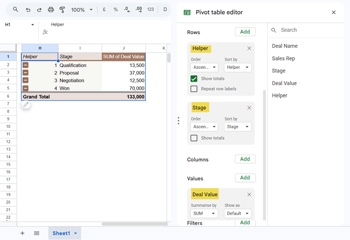
The Pivot Table is now sorted in the required custom order. The only thing left is to hide the Helper row grouping. We’ll take care of that in the next step.
Step 3: Clean Up the Pivot Table Layout
First, hide column H. Click the H column header, right-click it, and choose Hide column.
When you do so, the Grand Total label in the last row is also hidden because it is in column H.
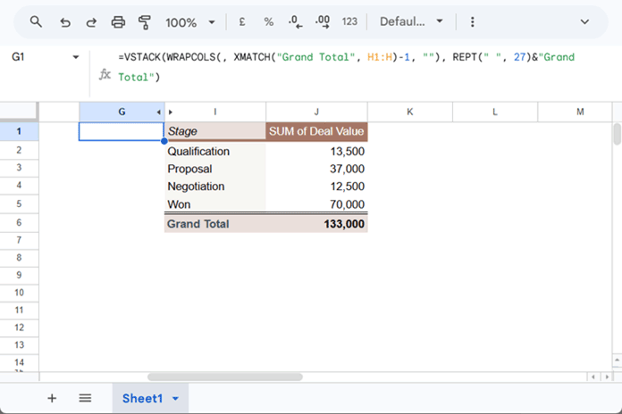
We can restore the label by recreating it in an empty column (column G in this example).
In cell G1, enter the following formula:
=VSTACK(
 WRAPCOLS(, XMATCH("Grand Total", H1:H) -1, ""),
 REPT(" ", 27)&"Grand Total"
)
If necessary, increase or decrease 27 to align the Grand Total label with the total value in the adjacent column.
How the Formula Works
Here’s how the formula works:
XMATCHfinds the position of Grand Total in the hidden column.WRAPCOLScreates the required number of blank cells.VSTACKplaces the recreated Grand Total label beneath those blank cells.REPT(" ", 27)adds leading spaces to align the label with the Pivot Table.
That’s it! Your Pivot Table rows are now sorted in the required custom order while maintaining a clean layout.
Sort Pivot Table Rows in Custom Order with Additional Row Fields
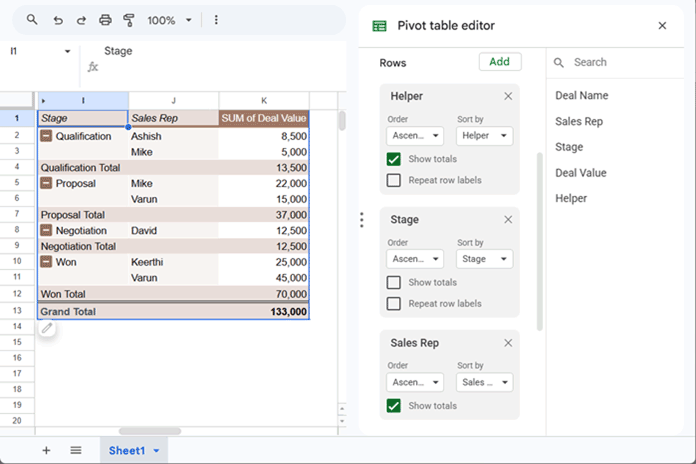
Adding additional row fields doesn’t affect the custom sort order, provided they’re placed below the Stage field in the Rows section.
For example, you can add Sales Rep or Deal Name immediately below the Stage field in the Rows section of the Pivot Table editor, not before it.
For example, adding Sales Rep below Stage produces the following Pivot Table.
Frequently Asked Questions
Does the custom sort order update when my dataset changes or grows?
Yes. The helper column formula expands automatically as new rows are added. As long as your Pivot Table uses the complete dataset (or a sufficiently large range), the custom sort order updates automatically.
How do I sort Pivot Table columns in a custom order?
A similar helper column formula is used, but the Pivot Table configuration and the formula used to restore the Grand Total label are different.
For the complete steps, see my related tutorial, How to Sort Pivot Table Columns in Custom Order in Google Sheets.
Conclusion
Sorting Pivot Table rows in a custom order may seem complicated at first, but the helper column approach is reliable and fully dynamic.
Instead of copying the Pivot Table as values into another range and manually rearranging the rows, or recreating the summary using functions such as QUERY or SUMIFS, you can let the Pivot Table maintain the required workflow order automatically as your source data changes.