How to Sort and Filter Pivot Tables in Google Sheets (Complete Guide)

Sorting and filtering are two of the most useful techniques for analyzing data in a Pivot Table in Google Sheets. You can further extend these capabilities using a few custom techniques.

After summarizing your data, you often need to organize the results to identify top-performing products, lowest-sales regions, or rows that meet specific conditions.

Google Sheets provides several built-in options for sorting and filtering Pivot Table results. However, advanced tasks—such as sorting in a custom order, filtering multiple values, or displaying only the top results with tie-breaking rules—require helper columns or custom formulas.

This guide brings together tutorials that explain how to sort, filter, and rank Pivot Table data in Google Sheets.

Table of Contents

Sorting Pivot Tables in Google Sheets

Sorting helps organize Pivot Table results so the most important information appears first. You can sort rows and columns by field values, summarized values, or custom criteria.

Google Sheets Pivot Table editor showing Sort by options for row and column fields

Sort Pivot Tables by Values

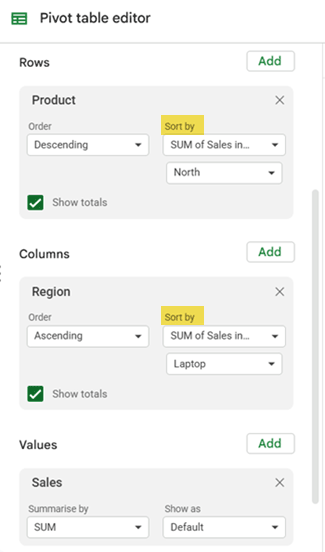
You can sort row and column fields by their field values or by summarized values. Depending on the Pivot Table layout, summarized values can include Grand Totals or the values for individual rows or columns.

See the tutorial: How to Sort a Pivot Table by Value in Google Sheets

Sort Pivot Table Columns in a Custom Order

Google Sheets does not provide a built-in option to display Pivot Table columns in a custom order. If you want a specific order (for example, North → East → South → West), you must use a helper column to define the custom sort order.

See the tutorial: How to Sort Pivot Table Columns in Custom Order in Google Sheets

Sort Pivot Table Rows in a Custom Order

Google Sheets lets you sort Pivot Table rows by field values or summarized values. If you need a completely custom sequence, you can achieve it using a helper column.

See the tutorial: How to Sort Pivot Table Rows in Custom Order in Google Sheets

Sort Pivot Table Rows by the Second Column

When a Pivot Table contains multiple row fields, Google Sheets always gives the first row field the highest sorting priority. As a result, sorting by the second row field may not produce the expected order.

A helper column can be used to assign a custom sort order to the first row field, allowing the Pivot Table rows to be effectively sorted by the second row field.

See the tutorial: How to Sort Pivot Table Rows by Second Column in Google Sheets

Filtering Pivot Tables in Google Sheets

Filtering lets you control which records appear in the Pivot Table results, helping you focus on the data that matters.

Google Sheets Pivot Table editor showing filter options for Pivot Table fields

Filter Multiple Values in a Pivot Table

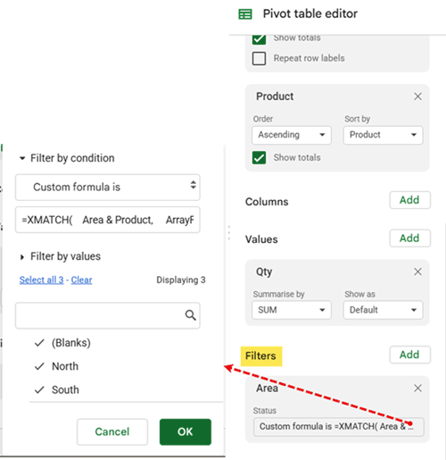
Google Sheets Pivot Tables allow only a single text condition in the built-in filter. While you can manually exclude multiple items using Filter by values, more flexible conditions—such as excluding multiple text strings dynamically—require a custom formula using REGEXMATCH or similar matching functions.

See the tutorial: Filter Multiple Values in Pivot Table in Google Sheets

Filter Pivot Table Rows by Total Values

Sometimes you need to filter Pivot Table rows based on summarized totals rather than individual records. For example, you may want to display only products whose total sales exceed a specific value.

This can be achieved using custom formulas such as SUMIF or COUNTIF within the Pivot Table filter settings.

See the tutorial: How to Filter by Total in Google Sheets Pivot Tables

Ranking Pivot Table Results (Top and Bottom Values)

Another useful technique is filtering Pivot Tables to display only the highest or lowest values, making it easier to identify the best or worst performers.

Filter the Top 10 Items in a Pivot Table

Google Sheets does not include a built-in Top 10 filter like Excel. However, you can achieve the same result using a custom ranking formula. The method also supports four tie-breaking modes (0, 1, 2, and 3), giving you control over how ties are handled.

See the tutorial: How to Filter Top 10 Items in a Google Sheets Pivot Table

Filter the Bottom 10 Items in a Pivot Table

You can also display the lowest values in a Pivot Table using a similar approach. This method supports the same four tie-breaking modes (0, 1, 2, and 3) and helps identify low-performing products, regions, or other categories.

See the tutorial: Filter the Bottom 10 Items in a Pivot Table in Google Sheets

Filter the Top Values Within Each Group in a Pivot Table

Sometimes you may want to display the top results within each group—for example, the top three products in each region. This requires a custom ranking formula applied through the Pivot Table filter.

The formula follows Excel’s Pivot Table behavior, returning the highest N values along with any duplicates of the Nth-ranked value.

See the tutorial: Filter the Top 3 Values in Each Group in a Pivot Table in Google Sheets

Conclusion

Sorting and filtering are essential for making Pivot Tables easier to analyze. While Google Sheets includes built-in options for many common tasks, advanced requirements often require helper columns or custom formulas.

The tutorials above cover techniques for:

Sorting Pivot Tables by summarized values
Creating custom row and column sort orders
Sorting rows by secondary fields
Filtering multiple values
Filtering by summarized totals
Displaying top or bottom results
Ranking items within groups

By combining these techniques, you can turn a basic Pivot Table into a more powerful data analysis tool.

If you’re new to Pivot Tables, you may also want to explore the other guides on this site covering Pivot Table basics, calculations, and formatting techniques in Google Sheets.