Pivot Table Formatting, Output & Special Behavior in Google Sheets

Pivot Tables in Google Sheets are powerful—but they can get tricky once you move beyond basic summaries. Need to drill down dates, extract totals, fill blanks with zeros, apply conditional formatting, or handle hidden rows? Some of these aren’t obvious—and a few aren’t directly supported at all.

This hub brings advanced Pivot Table tricks together in one place. Each section tackles a real-world challenge and walks you through step-by-step solutions.

If you use Pivot Tables regularly, this guide will give you full control over how your data is grouped, displayed, extracted, and filtered—without having to touch your source data.

Table of Contents

Drill Down Date Fields Without Extra Columns

When working with financial statements, sales data, or transaction logs, dates are often stored in a single column. Yet, for analysis, you may want to view the same data year-wise, quarter-wise, or month-wise.

Instead of adding helper columns or creating multiple Pivot Tables, Google Sheets allows you to define a date hierarchy directly inside the Pivot Table. By grouping the date field and adding multiple date levels, you can drill down and drill up dynamically using expand/collapse controls.

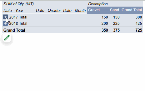
Drill down and expand date fields in a Pivot Table in Google Sheets using year, quarter, and month grouping

👉 Read the full tutorial: Drill Down in Pivot Table in Google Sheets (Date Field)

This is especially useful for:

Financial year analysis
Quarterly performance tracking
Monthly summaries from daily data

Extract Subtotal and Grand Total Rows Dynamically

To extract values from a Pivot Table, the GETPIVOTDATA function is usually the go-to solution. Other functions may work in some cases, but they can break when the Pivot Table expands or shrinks as your source data changes.

However, there’s a challenge when dealing with subtotal or grand total rows. Using GETPIVOTDATA here often results in deeply nested, repetitive formulas that are difficult to maintain.

A more reliable and dynamic approach is to treat the Pivot Table output as a structured range and extract rows containing “Total” using standard formulas. This method allows subtotal and grand total rows to move freely as the Pivot Table grows or changes, without breaking your calculations.

👉 Read the full tutorial: Extract Total and Grand Total Rows From a Pivot Table in Google Sheets

This technique is ideal when:

You need totals in dashboards or reports
Source data changes frequently
You want formulas that don’t break when rows shift

Exclude Manually Hidden Rows from Pivot Table Calculations

Filtering data using slicers or Pivot Table filters works as expected—but manually hidden rows are still included in Pivot Table calculations. Google Sheets does not provide a built-in option to exclude them.

The only reliable workaround is to use a helper column that dynamically flags visible and hidden rows. You can then filter the Pivot Table using this flag so hidden rows are excluded from totals and aggregations.

👉 Read the full tutorial: How to Exclude Manually Hidden Rows from a Pivot Table in Google Sheets

This approach is useful when:

You hide rows for privacy or review
You want reports to ignore hidden data
You need non-destructive exclusion without deleting rows

Fill Empty Pivot Table Cells with Zero (0)

Filling empty cells with 0 in a Pivot Table in Google Sheets isn’t straightforward. Why would you even need this?

I recall a client who requested empty cells be filled with 0 in invoices—likely to prevent misinterpretation, avoid manual manipulation, or comply with company policy.

By default, blank cells in Pivot Tables represent missing records, not zeros. Automatically converting blanks to 0 can be misleading, which is why Google Sheets doesn’t offer a built-in option.

However, if your reporting requires zeros—for charts, comparisons, or exports—you can generate the missing records using formulas and append them to your source data. Once those records exist, the Pivot Table will naturally fill empty cells with 0.

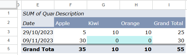
Google Sheets Pivot Table with blank cells replaced by 0 for consistent reporting

👉 Read the full tutorial: How to Fill Empty Cells with 0 in Pivot Table in Google Sheets

This method is helpful when:

Charts require consistent numeric values
You compare categories across dates
You export Pivot Table results to other systems

Apply Conditional Formatting That Stays Inside the Pivot Table

Conditional formatting in Pivot Tables is tricky because the table size changes dynamically. Applying formatting to fixed ranges often results in highlights spilling outside the Pivot Table—or missing new data.

By using custom formulas based on GETPIVOTDATA, you can dynamically restrict conditional formatting to:

Specific row labels
Aggregated values meeting defined conditions

The formatting automatically expands and contracts with the Pivot Table.

👉 Read the full tutorial: Conditional Formatting for Pivot Tables in Google Sheets

This is ideal for:

Highlighting key categories
Flagging high or low aggregated values
Creating readable, self-updating reports

When This Hub Is Useful

This hub is for users who are comfortable with Pivot Tables and want full control over their output, formatting, and special behaviors.