Excluding manually hidden rows from a Pivot Table in Google Sheets is not straightforward—but it is possible with a workaround.
Google Sheets does not provide a built-in option to ignore manually hidden rows in Pivot Tables. To achieve this behavior, you must use a helper column powered by a dynamic array formula that detects hidden rows and flags them automatically.
Once flagged, you can use the Pivot Table Filters to exclude those rows from the report.
This guide covers an advanced workaround and is relevant only when rows are manually hidden—not when filters or slicers are used.
This tutorial is part of the hub Pivot Table Formatting, Output & Special Behavior in Google Sheets and covers an advanced Pivot Table limitation. It is relevant only when rows are manually hidden, not when filters or slicers are used.
How This Workaround Works (Overview)
The process involves three steps:
- Add a helper column to your source data.
- Use a dynamic array formula to identify hidden vs visible rows.
- Filter the Pivot Table using that helper column.
The helper column dynamically updates whenever rows are hidden or unhidden, ensuring the Pivot Table reflects only visible rows.
Why Pivot Tables Ignore Manually Hidden Rows in Google Sheets
In Google Sheets, data can be hidden in two fundamentally different ways:
1. Systematic filtering (partially supported)
- Data → Create a filter
Filters applied directly to the source range do not affect Pivot Tables. - Data → Add a slicer
A slicer can filter a Pivot Table only when it is explicitly connected to that Pivot Table.
These methods hide rows systematically, but only slicers—when linked—can control Pivot Table output.
2. Manual row hiding (not supported)
- Right-click → Hide row
Manually hidden rows are still treated as valid data by Pivot Tables. As a result, their values are included in calculations unless you apply a workaround.
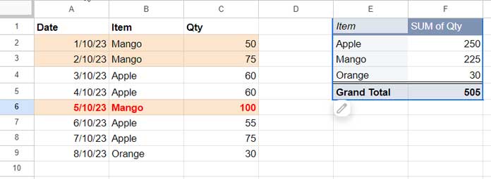
Example Scenario
Suppose your source data contains the item “Mango” in three rows with values:
- 50
- 75
- 100
Total shown in the Pivot Table: 225
If you manually hide the row containing 100, the Pivot Table still includes it—unless you intervene.
Using the helper-column method described below, the Pivot Table updates correctly and displays 125 instead.
When Would You Need This?
This technique is useful when you need to:
- Exclude sensitive data from reports
- Temporarily hide outdated entries without deleting them
- Generate printable or PDF reports that omit specific rows
- Preserve raw data while controlling report output
How to Exclude Manually Hidden Rows Using a Helper Column
To see a live example, make a copy of the sample sheet below:
Sample Setup
- Source data: columns A:C
- Pivot Table starts at E1
- Helper column will be added in column D
Create the Pivot Table by selecting columns A:C and clicking Insert → Pivot table
If you are new to Pivot Tables, see Google Sheets Pivot Table Basics & Setup for a step-by-step introduction.
Helper Column Requirements
Choose a column that:
- Is blank
- Immediately follows the source data
- Corresponds to a Row field in the Pivot Table
In this example, column D meets all criteria.
Helper Column Formula
In cell D1, enter the following formula:
=VSTACK("Hidden Flag", BYROW(B2:B, LAMBDA(row, SUBTOTAL(103, row))))
What this does:
- Returns 1 for visible rows
- Returns 0 for manually hidden rows
- Automatically expands with your data
- Inserts the header “Hidden Flag” in D1
Which Column Should You Reference?
Use the column that corresponds to the Row field in your Pivot Table.
In this example:
- The Row field is Item
- Item values are in column B
- Therefore, the formula references B2:B
Add the Helper Column to the Pivot Table
- Hover over the Pivot Table
- Click the Edit (pencil) icon
- Update the data range from A:C to A:D
- Click outside the range field (do not press Enter)
- Click OK
Filter the Pivot Table to Exclude Hidden Rows
- In the Pivot Table editor, click Add next to Filters
- Select Hidden Flag
- Open the filter dropdown
- Uncheck 0
- Click OK
Close the editor.
Now, when you manually hide any row, the Pivot Table updates automatically and excludes that data.
Important Limitation to Be Aware Of
If your source data is filtered using a slicer, this method will also exclude those rows.
➡️ Do not use slicers or filters on the source data when applying this workaround.
Note: If the Pivot Table does not update immediately after hiding or unhiding rows in Google Sheets, cut and paste the helper-column formula to force a refresh.
Conclusion
Google Sheets Pivot Tables cannot exclude manually hidden rows by default.
The helper column method described here is currently the only reliable solution for excluding manually hidden rows while preserving the underlying data.
Although it requires an extra column, it provides precise control over Pivot Table output—especially in advanced reporting and data-privacy scenarios.


