In this tutorial, I’ll explain how to create a Pivot Table report in Google Sheets. It contains all the essential steps you need to understand pivot tables and use them confidently for data analysis.

You can quickly summarize large datasets using Pivot Tables in Google Sheets—without writing complex formulas.

Pivot Tables and the QUERY function are the two most powerful tools in Google Sheets for grouping and aggregating data. A Pivot Table is created through the menu, while QUERY is a worksheet function. Both have their own strengths.

If you work regularly with spreadsheets, knowing how to create a Pivot Table in Google Sheets is an essential skill.

Whether you’re using Microsoft Excel or Google Sheets, Pivot Tables remain one of the most effective ways to analyze data.

This tutorial is part of our Google Sheets Pivot Table Tutorial, which covers pivot table basics, setup, and advanced date-grouping techniques.

Purpose of Creating a Pivot Table Report in Google Sheets

The primary purpose of a Pivot Table is to analyze large datasets efficiently.

With Pivot Tables, you can:

• Summarize data dynamically (reports update automatically when source data changes)
• Group and aggregate values with just a few clicks
• Avoid writing manual formulas for common calculations

In some cases, built-in aggregations may not be enough. When that happens, you can use calculated fields inside Pivot Tables to apply custom formulas—an option often required by advanced users.

Using Pivot Tables to Summarize Data in Google Sheets

To understand how Pivot Tables work, we’ll use sample data.

Since creating sample data manually takes time, we’ll use a ready-made sample dataset provided by Google, which is perfect for learning and experimentation.

Sample Sheet

Open the sample spreadsheet using the link provided. Click “Use Template” to create a copy in your Google Drive.

This dataset contains a list of college students with the following columns:

• Student Name
• Gender
• Class Level
• Home State
• Major
• Extracurricular Activity

We’ll use Class Level and Major to create our Pivot Table report.

Our goal is to summarize the data to find how many students (Senior, Junior, Freshman, etc.) are enrolled in each subject.

Steps to Create a Pivot Table Report in Google Sheets

Step 1: Select the Source Data

Select the entire dataset.

On Windows, a quick method is:

• Click the first cell
• Press Ctrl + Shift + Right Arrow (selects the row)
• Press Ctrl + Shift + Down Arrow (selects the full range)

Alternatively, you can select the range using your mouse.

Then go to:

Insert → Pivot table → New sheet → Create

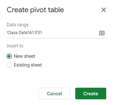
The Existing sheet option allows you to place the Pivot Table in a specific cell on any existing sheet.

A new sheet opens with the Pivot table editor on the right.

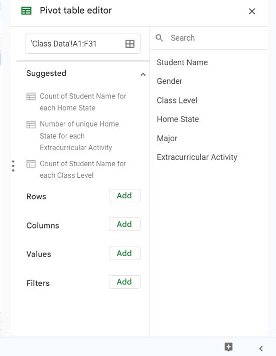
Note: If you close the Pivot Table editor panel, you can open it again by hovering over the Pivot Table and clicking the pencil icon at the bottom-left corner. This will reopen the editor so you can add or remove rows, columns, values, and filters.

Step 2: Add Rows and Columns

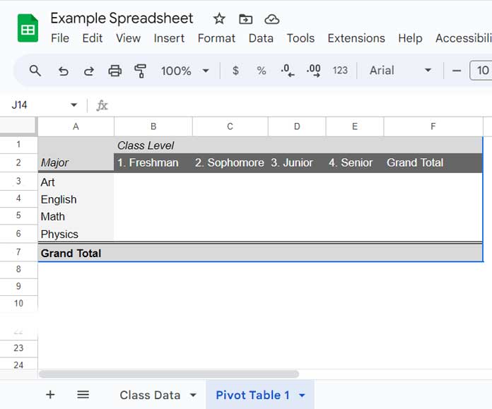
We want to show subjects (Majors) in rows and Class Levels in columns.

• Under Rows, click Add → select Major
• Under Columns, click Add → select Class Level

At this stage, the Pivot Table structure is in place, but it doesn’t yet show values.

Step 3: Add Values (Counts)

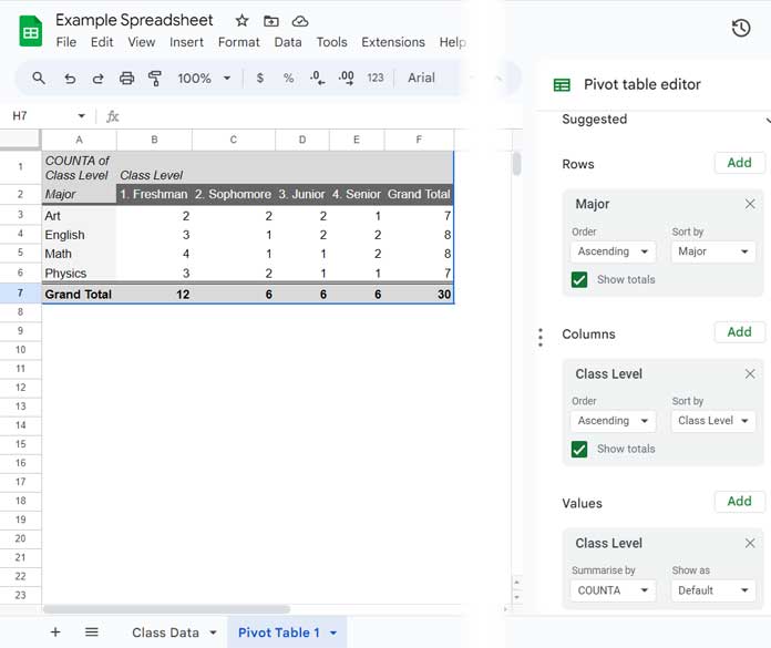
Now we need to count how many students fall under each class level for each subject.

• Under Values, click Add → select Class Level
• Set Summarize by to COUNTA

Why COUNTA?

Because the Class Level column contains text values (Senior, Junior, etc.), not numbers.

Your Pivot Table report is now complete.

Despite the number of steps, this entire process usually takes 2–3 minutes once you understand the logic.

Refreshing the Pivot Table Report

The Pivot Table was created from the range A1:F31.

• Any edits within this range update the Pivot Table automatically
• New rows added outside this range will not appear in the report

How to Handle Expanding Data

You have two reliable options:

Option 1: Use an Open-Ended Range

Create the Pivot Table using an open-ended range such as A1:F instead of a fixed range. This ensures that newly added rows are automatically included in the Pivot Table.

Using an open-ended range may initially introduce blank rows in the Pivot Table. While you can remove these by unchecking Blanks in the filter, doing so may prevent newly added rows from appearing in the Pivot Table later.

Recommended approach to filter empty rows without breaking future updates:

1. In the Pivot table editor, add the row field (for example, Major) under Filters.
2. Click the added filter field.
3. Choose Filter by condition → Custom formula is.
4. Enter the formula: =Major<>""
5. Click OK to apply the filter.

This condition explicitly excludes empty rows from the Pivot Table while still allowing the source range to expand automatically.

Option 2 (Recommended): Convert Source Data to a Table

The most reliable way to ensure your Pivot Table always includes new data is to convert the source range into a table before creating the Pivot Table report.

When you create a Pivot Table from a table, Google Sheets automatically expands the source range as new rows are added.

Best practice:

• Convert the source data to a table first
• Then create the Pivot Table using the table as the source

Related: Converting a Range to a Table and Vice Versa in Google Sheets

If you convert the range to a table after creating the Pivot Table:

1. Select the existing Pivot Table.
2. Open the Pivot table editor.
3. In the Data range field, replace the original cell range (for example, A1:F) with the table name (for example, Table1).
4. Press Enter to apply the change.

Once the Pivot Table uses the table name as its source, it will automatically include future rows added to the table.

Final Thoughts

Creating a Pivot Table report in Google Sheets is one of the fastest ways to summarize and analyze data.

Once you master this foundation, you can move on to:

• Date grouping
• Week-wise analysis using helper columns
• QUERY-based reporting for advanced use cases

➡️ For a complete learning path, refer back to the Google Sheets Pivot Table Tutorial hub, where all related guides are organized in one place.